greenhouse gas research in agriculture

For sustainability environment: some determinants of greenhouse gas emissions from the agricultural sector in EU-27 countries

• Research Article
• Open access
• Published: 23 April 2024

Cite this article

You have full access to this open access article

• Hasan Gökhan Doğan   ORCID: orcid.org/0000-0002-5303-1770 1 &
• Mustafa Kan   ORCID: orcid.org/0000-0001-9198-5906 1  

Climate events significantly affect the lives of not only humanity but also all living things. Just as transformation in the ecosystem affects sectors, all sectors also transform the ecosystem. It is stated that the agricultural sector is at the root of the deterioration in the ecosystem due to the effect of intensive agriculture after the green revolution. It can be stated that, with an understanding far from the concept of sustainability, the foodstuffs and their waste produced in the agricultural sector are considered among the causes of climate change, which is now concentrated on the whole world in the third millennium. In this study, the effect of N 2 O gas released from produce residues and the release of enteric fermentation on the level of CO 2 released from agricultural-food systems was investigated using advanced econometric models. The findings reveal that both factors are effective. However, it can be stated that the effect of N 2 O gas released from the produce residues is greater. Suggestions such as improving feed rations and maintaining herd management strategies within certain patterns to reduce the level of enteric fermentation may contribute to the process. In produce residue management, turning waste into compost and expanding bioenergy power plants will ensure both waste disposal and resource continuity in generating energy. Otherwise, the decreasing resources in the world may come to an end, and there will be disruptions and problems in the agricultural sector, as in all sectors. Considering the increasing world population, it is inevitable that food supply security may be endangered and the hunger problem may reach an irreversible level.

Avoid common mistakes on your manuscript.

Introductıon

Climate change is one of the most serious problems that threaten the future of humankind. In a study conducted on global risks, it is stated that the top three most important risks in the long term are failure to achieve success in the fight against climate change and the resulting natural disasters (World Economic Forum (WEF) 2023 ). Greenhouse gasses in the atmosphere, which are shown to be one of the main causes of climate change, started to increase after the Industrial Revolution that started in the 1750s, and the Intergovernmental Panel on Climate Change (IPCC) states that these increases are definitely caused by human activities (IPCC 2013 ). In addition to occurring naturally, greenhouse gasses occur because of various human activities (Köknaroglu and Akünal 2010 ). Energy is a sector that plays the largest role in greenhouse gas emissions (Fig.  1 ).

Share of sectors greenhouse gas emissions (%) (FAO 2023a , b )

Agriculture, a sector that significantly affects greenhouse gas emissions, is a sector that is affected by climate change. Within the scope of the UN Sustainable Development Goals, “SDG 13: Climate action” is directly related to agricultural production (United Nations 2023 ). Sustainable land use, the future of food, the future of consumption, etc. Within the framework of the discussions, it is recommended that new agricultural practices and technologies be developed in the fight against climate change. On the other hand, the development of agricultural practices that contribute to the reduction of GHG emissions will contribute to the mitigation side of the fight against climate change (Kara and Yereli 2022 ).

Considering that approximately 2.5 billion people in developing countries earn their living from agriculture, it is clear to what extent climate change will threaten human welfare and agricultural production. Agriculture is a basic and strategic sector known for its contribution to the nutrition of people all over the world, national income and employment, providing raw materials and capital to the industrial sector, and its contributions to biodiversity and ecological balance (Doğan et al. 2015 ). In parallel with the ever-increasing world population, the need for food is increasing day by day. Greenhouse gasses such as CO 2 (carbon dioxide), CH 4 (methane), and N 2 O (nitrous oxide), which occur as a result of agricultural activities (energy consumption, plant and animal production, fertilization, pesticide use, etc.), are considered among the causes of climate change (Akalın 2014 ). Important agricultural activities that affect greenhouse gas emissions are presented in Fig.  2 .

Share of agricultural activities in climate change (%) (FAO 2023a , b )

Among the effects of agricultural activities on climate change, main activities such as energy consumption, production, animal husbandry, fertilization, and spraying, as well as N 2 O release resulting from waste in plant production and CH 4 release resulting from enteric fermentation because of livestock activities, are also important factors (Fig.  2 ). When the figures for 2021 are examined, it is stated that the most important contributors to greenhouse gas emissions are CO 2 emissions from deforestation and methane (CH 4 ) emissions from the enteric fermentation of ruminant livestock (2.9 gigaton CO 2 eq each). This represents 40% of the total agri-food system. Other important components are CH 4 emissions from animal manure (manure management, soil application, and manure deposition) and agri-food system waste disposal, each around 1.3 Gt CO 2 eq (FAO 2023a , b ). Among the greenhouse gasses, N 2 O has a 265 times stronger effect on global warming than CO 2 (IPCC 2013 ). In the last 200 years, atmospheric concentrations of important greenhouse gasses, CO 2 , CH 4 , and N 2 O, have increased significantly. El-Fadel and Massoud ( 2001 ) stated that the increase in greenhouse is caused by the production and use of fossil fuels, agricultural activities, and industrial activities. According to the (IPCC 2007a , b ), the global warming potential values of CO 2 , CH 4 , and N 2 O gasses over a 100-year period are reported to be 1, 21, and 310 carbon dioxide equivalents, respectively. Greenhouse gasses such as CH 4 and N 2 O, which are produced by waste and enteric fermentation, are gaining importance as gasses that contribute significantly to global warming because of their high global warming potential. Given that these gasses originate from enteric fermentation and agri-food systems, there are many proposals to reduce emissions. However, reducing production in the face of increasing food demand will be a major challenge. However, without a reduction in production, it is better to manage wastes and emissions properly and to create policies to do so. This is what this research focuses on.

This study aims to evaluate the impact of produce residues and greenhouse gas emissions resulting from enteric fermentation on the emissions released within the scope of the agricultural food system in the EU 27 countries.

Materıal and method

The symbols, units, and data sources regarding the share of emissions released from agriculture-food systems in total emissions, the amount of N 2 O released from produce residues, and the amount of CO 2 emissions resulting from enteric fermentation between 2000 and 2020 for the EU-27 countries are given in Table  1 . In the third millennium, while developing policies to respond to the nutritional opportunities of the growing population, policies have also been sought in terms of environmental pressure and cost. Therefore, post-2000 research is gaining importance. In these policies, the EU is decisive. Because many economically developed countries of the world are located in this region. Since it is a regional structure, it is an important formation both agriculturally and commercially.

For the EU-27 countries determined as the research area, a panel data set was used using the variables given in Table  1 . After the dataset was created, the “dog-log” model in semi-logarithmic form was preferred to provide interpretation opportunities because the unit of the dependent variable was proportional. Equation e = ꞵit/Y was used to determine the elasticities of the coefficients obtained in the dog-log (semi logarithmic function) models. Because, logarithmic functions allow exponential functions to be linearized and interpreted as percentages. However, in our equation, the dependent variable is already included in the model as a percentage. The functional relationship between the variables can be expressed as in Eq.  1 .

After the hypothetically put forward functional relationship, the following panel data analyses were carried out to determine the impact levels of the emissions released from agricultural-food systems on the share of total emissions:

Panel unit root test

Panel toda–yamamato causality test, panel ardl test.

In panel data econometrics, both time and differences between units can be examined together (Cameron and Trivedi 2005 ). Panel data creates a dataset consisting of t time and k variables for n cross-sections, thus allowing time and group effects to be included in the model. As in time series analysis, whether variables contain unit roots in panel data models should be investigated. Engle and Granger ( 1987 ) demonstrated that if the series are not stationary at their levels, the coefficients obtained from classical regression will be invalid. When working with a non-stationary series, the long-term relationship between the series disappears, and the relationship between the series does not reflect the truth. Many unit root tests are used in practice to investigate the stationarity of a series. The first-generation tests developed by Maddala and Wu ( 1999 ), Levin et al. ( 2002 ), Hadri ( 2000 ), Choi ( 2001 ), and Im et al. ( 2003 ) can be shown as an example of unit root tests (Doğan 2018 ).

In this study, panel unit root tests introduced by Levin et al. ( 2002 ) and Im et al. ( 2003 ) were preferred. Unlike the others, this test considers the heterogeneous structure in the panel data set as it first tests whether there is a unit root for each horizontal section separately to obtain panel-specific results (Güloğlu and İspir 2009 ).

where X represents the constant and/or deterministic trend variables.

The ARDL bounds test approach allows co-integration testing with series that are not stationary at the same level (Pesaran and Shin 1995 ; Pesaran et al. 2001 ). The advantage of the ARDL approach is that co-integration testing can be performed without considering the degree of integration of the variables. In this study, the pooled mean group (PMG) estimator developed by Pesaran et al. ( 1999 ) was used to estimate long-term coefficients. The PMG estimator allows constant error term variances and short-run coefficients to vary. On the other hand, it allows the assumption of heterogeneity for short-term coefficients and homogeneity for long-term coefficients. The model created by following the ARDL approach developed by Pesaran et al. ( 1999 ) and using the PMG estimator is given in Eqs. 3 , 4 , and 5 .

In Eqs. 3 , 4 , 5 , Δ refers to the difference processor, and m refers to the lag length. Information criteria such as AIC, SC, FPE, and HQ are used to determine the lag length. Here, the lag length that provides the smallest critical value is determined as the lag length of the model (Doğan 2018 ).

In this study, the Wald test (MWALD) recommended by Toda and Yamamoto ( 1995 ) was used. The Toda–Yamamoto Test ignores the I(0) and I(1) incompatibility between the series and the assumption of co-integration (Zapata and Rambaldi 1997 ; Wolde-Rufael 2004 , 2005 ). This eliminates the difficulties and nativities that may arise in other causality tests. The MWALD test minimizes the risks related to the co-integration orders of the series by creating a VAR model according to the levels of the variables (Mavrotas and Kelly 2001 ). In this process, the appropriate “k” lag is determined, the maximum stationarity level dmax is determined, and the VAR model is solved with the lag k  + dmax (Rambaldi 1997 ; Zapata and Rambaldi 1997 ). The results obtained have an asymptotic distribution and are not biased. Notations for the Toda–Yamamoto causality test are given in Eqs.  6 , 7 , and 8 . The causality relationship and direction were determined by analyzing the following VAR system adapted for this study.

Models are analyzed by applying the “Seemingly Unrelated Regression” (SUR) procedure.

Empirıcal results

Descriptive statistics for the variables included in the study are given in Table  2 .

LLC and IPS unit root test results for the ⅄ , ₱ , and ℇ variables used in this study are given in Table  3 .

When the LLC and IPS unit root test results for the variables are examined, it can be said that ⅄ contains a unit root at I(0) and is stationary at the I(1) level compared with LLC and IPS. ₱ is stationary at both I(0) and (1) levels according to LLC and IPS, and ℇ has a unit root at I(0) level according to LLC and I(1) level according to IPS. It can be stated that it contains but is stationary at the I(1) level.

The results of the Toda–Yamamato causality test, which was constructed with VAR (vector auto regression) systems and considered the k  + dmax lag length and stationarity level, are given in Table  4 . Causality was analyzed in one way. Since the main purpose of this study is to reveal the severity of the parameters affecting the share of CO 2 released from agricultural food systems, one-way analysis results are expressed.

When the results of the Toda-Yamamato causality test were examined, causality was determined from the amount of N 2 O released from produce residues to the share of the agricultural-food systems in total emissions and from enteric fermentation to the share of the CO 2 level released from the agricultural-food systems. The severity of this relationship is expressed by the panel ARDL results in Table  5 .

After determining whether the variables were affected by their previous values with the unit root test, the ARDL test was performed to reveal their long-term relationships. The ARDL test allows investigating the relationship of co-integration in the long run, regardless of whether the variables examined are stationary at the same level. ARDL long-term and short-term test results are given in Table  5 .

When the results of ARDL (1,2,2) are examined, both variables examined on the share of CO 2 emissions from agricultural-food systems in total emissions are statistically significant in the long term. When the amount of N 2 O released from produce residues increases by 1%, the share of CO 2 released from agricultural food systems increases by 0.05%. Conversely, when the amount of CO 2 resulting from enteric fermentation increases by 1%, the share of CO 2 released from agricultural food systems increases by 0.01%. In the short term, it can be said that the effect of the N 2 O level released from the residues in the current period and the t –1 period is statistically significant. When the sources of agricultural CO 2 emissions are examined, it can be stated that the N 2 O level released from produce residues and the CO 2 level resulting from enteric fermentation are essential (FAO 2023a , b ).

Recommandatıon and conclusıon

Today, when climate change is felt more and more each day, countries are making commitments to reduce greenhouse gas emissions and develop policies and strategies on this issue (Bulut et al. 2023 ). The European Union, the world’s largest economic and political union, creates significant impacts all over the world with the policies it implements. One of these is the agricultural sector. It is known that 60% of the methane released from anthropogenic sources is released from agricultural activities, whereas 25% is released from enteric fermentation (Singh and Singh 2012 ; Keser and Kutay 2021 ). EU countries, which try to direct agriculture and rural areas through the Common Agricultural Policy, are taking important steps toward becoming a carbon–neutral and environmentally friendly community in the future. The effect of emissions resulting from produce residues and enteric fermentation on the greenhouse gas emissions released from the agricultural food system was found to be statistically significant in the short and long term. The findings obtained also coincide with reality. It can be said that livestock activities are essential in reducing greenhouse gas emissions caused by the agricultural sector. There is an intense release from both enteric fermentation and animal fertilizers. However, enteric fermentation has a greater impact. Various strategies can be put forward to combat this situation. First feeding is essential in animal husbandry activities. This is a paradox where, on the one hand, there is the efficiency and quality to be achieved per unit animal, and on the other hand, there are measures to be taken against the environmental costs. However, it is not insoluble. There are studies that recommend the use of various additives (yeast, probiotic, organic acid, etc.) to better utilize the energy of the feed and reveal their methane-reducing effect (Altan and Acar 2022 ). As the carbohydrate and fat content in the diet increases, methane emissions can be reduced (Moss et al. 2000 ; Meral and Biricik 2013 ). Additionally, as the amount of roughage increases in the ration of animals consuming high amounts of dry matter, methane emissions also increase (McAllister et al. 2011 ). On the other hand, within herd management strategies, improving genetic materials and removing unproductive animals from herds can have a positive effect on ensuring optimum efficiency. This also can reduce methane (Eckard et al. 2010 ; Pragna et al. 2018 ). In countries where livestock activities are intensive, continuing such practices with established policies may be beneficial in terms of adaptation and reduction. Produce residue management is another important issue. GHG emissions released from produce residues need to be managed. Otherwise, it may lead to the deterioration of the chemical structure of the atmosphere at both local and regional levels (Bencs et al. 2008 ). Although burning waste is prohibited in many countries, it continues to be burned for various reasons (removal of weeds, field preparation for the next year, disease control, etc.) (Gadde et al. 2009 ). The monitoring and evaluation processes of waste management must be within the framework of legal legislation. Political sanctions should be applied. Turning waste into compost and using it for plant nutrition will not only be beneficial in reducing emissions but also contribute to reducing the gasses that can be released by reducing the use of chemical fertilizers. On the other hand, producers’ plants produce residues that can be used in biomass power plants to obtain low-emission energy. Although there are difficulties such as transportation and storage, they can be traded within the scope of the clean development mechanism. For sustainable agricultural production and a sustainable environment, the interaction between waste obtained from agricultural producers and energy power plant investors may be a way out.

Akalın M (2014) İklim Değişikliğinin Tarım Üzerindeki Etkileri: Bu Etkileri Gidermeye Yönelik Uyum ve Azaltım Stratejileri. Hitit Üniversitesi Sosyal Bilimler Enstitüsü Dergisi Sayı 2:351–357

Google Scholar  

Altan NN, Acar MC (2022) Ruminant Beslemede Enterik Metan Salınımını Azaltmaya Yönelik Stratejiler. 6th International Students Science Congress. (1).1–7 https://doi.org/10.52460/issc.2022.004

Bencs L, Ravindra K, deHoog J, Rasoazanany EO, Deutsch F, Bleux N, Berghmans P, Roekens E, Krata A, VanGrieken R (2008) Massand ionic composition of atmospheric fine particles over Belgium and their relation with gaseousairpollutants. J Environ Monitor 10(10):1148

Article   CAS   Google Scholar  

Bulut U, Ongan S, Dogru T, Işık C, Ahmad M, Alvarado R, Rehman A (2023) The nexus between government spending, economic growth, and tourism under climate change: testing the CEM model for the USA. Environ Sci Pollut Res 30(36):86138–86154

Article   Google Scholar  

Cameron AC, Trivedi PK (2005) Micro econometrics: methods and applications. Cambridge University Press, New York

Book   Google Scholar  

Choi In (2001) Unit root tests for panel data. J Int Money Finance 20(249):272

Demir P, Cevger Y (2007) Küresel Isınma ve Hayvancılık Sektörü. Veteriner Hekimler Derneği Dergisi, 78/1, S: 15–16, Ankara, Türkiye.

Doğan H (2018) Nexus of Agriculture, GDP, Population and climate change: case of some Eurasian countries and Turkey. Appl Ecol Environ Res 16(5):6963–6976

Doğan Z, Arslan S, Berkman A (2015) Türkiye’de tarim sektörünün iktisadi gelişimi ve sorunlari: tarihsel bir bakiş. Niğde Üniversitesi İktisadi Ve İdari Bilimler Fakültesi Dergisi 8(1):29–41

Eckard RJ, Grainger C, De Klein CA (2010) Options for the abatement of methane and nitrous oxide from ruminant production: a review. Livest Sci 130:47–56

El-Fadel M, Massoud M (2001) Methane emissions from wastewater management. Environ Pollut 114(2):177–185

Engle R, Granger CWJ (1987) Cointegration and error correction: representation estimation and testing. Econometrica 55(2):251–276

FAO (2023a) www.faostat.org.tr . https://www.fao.org/faostat/en/#data/EM/visualize

FAO (2023b) Agrifood systems and land-related emissions. Global, regional and country trends, 2001– 2021. FAOSTAT Analytical Briefs Series No. 73. Rome. https://doi.org/10.4060/cc8543en

Gadde B, Bonnet S, Menke C, Garivait S (2009) Air pollutant emissions from rice straw open field burning in India, Thailand and the Philippines. Environ Pollut 157:1554–1558. https://doi.org/10.1016/j.envpol.2009.01.004

Güloğlu B, İspir S (2009) Panel unit root test of purchasing power parity hypothesis in turkey in the light of new developments. Pamukkale University Department of Economics Publications. (in Turkish)

Hadri K (2000) Testing for stationarity in heterogeneous panel data. Econom J 3:148–161

Im KS, Pesaran MH, Shin Y (2003) Testing for unit roots in heterogeneous panels. J Econom 115(1):53–74

Intergovernmental Panel on Climate Change (IPCC) (2007) Changes in atmospheric constituents and in radiative forcing. Forster P, Ramaswamy V, Artaxo P, Berntsen T, Betts R, Fahey DW, Haywood J, Lean J, Lowe DC, Myhre G, Nganga J, Prinn R, Raga G, Schulz M, Van Dorland R. The Physical Science Basis. Contribution of Working Group I to the Fourth Assessment Report of the Intergovernmental Panel on Climate Change, New York, ABD.

IPCC (2007a) Climate change-ımpacts, adaptation and vulnerability. In: (Eds.: Parry, M.L., Canziani, O.F., Palutikof, J.P., van der Linden, P.J., Hanson, C.E.) Cambridge University Press, Cambridge, UK, pp. 976

IPCC (2007b) Climate Change 2007, Impacts, adaptation, vulnerability. https://www.ipcc.ch/pdf/assessment-report/ar4/wg2/ar4_wg2_full_report.pdf

IPCC (2013) Climate Change 2013: The Physical Science Basis. Working Group I Contribution to the Intergovernmental Panel on Climate Change Fifth Assessment Report, Stockholm

Kara KÖ, Yereli AB (2022) İklim Değişikliğinin Yönetimi ve Tarım Sektörü. Afet Ve Risk Dergisi 5(1):361–379

Keser O, Kutay HC (2021) Küresel Isınmaya Karşı Ruminantlarda Metan Emisyonunu Azaltmaya Yönelik Besleme Stratejileri. Türk Bilimsel Derlemeler Dergisi 2146–013214(2):138–159

Köknaroglu H, Akünal T (2010). Küresel Isınmada Hayvancılığın Payı ve Zooteknist Olarak Bizim Rolümüz, Süleyman Demirel Üniversitesi Ziraat Fakültesi Dergisi 5/1 s:67–75

Levin A, Lin CF, Chu CSJ (2002) Unit root tests ın panel data: asymptotic and finite sample properties. J Econometrics 108:1–24

Maddala GS, Wu S (1999) A comparative study of unit root tests with panel data and a new simple test. Oxf Bull Economics Stat 61:631–652

Mavrotas G, Kelly R (2001) Old wine in new bottle: testing causality between savings and growth. The Manchester School Supplement 97–105

McAllister A, Okine EK, Mathison GW, Cheng KJ (2011) Dietary, environmental and microbiological aspects of methane production in ruminants. Can J Animal Sci 76(2):231–243

Meral Y, Biricik H (2013) Metan Emisyonunu Azaltmak için Kullanılan Besleme Yöntemleri. VII. Ulusal Hayvan Besleme Kongresi (Uluslararası Katılımlı), 26–27 Eylül; Ankara

Moss AR, Jouany JP, Newbold J (2000) Methane production by ruminants: its contribution to global warming. Ann Zootech 49:231–253

Pesaran H, Shin Y (1995) An autoregressive distributed lag modelling approach to cointegration analysis. In: Strom S, Holly A, Diamond A (eds) Centennial Volume of Ranger Frisch. Cambridge University Press

Pesaran MH, Shin Y, Smith RJ (2001) Bound testing approaches to the analysis of long run relationship. J Appl Economet 16(3):289–326

Pesaran M, Shin Y, Smith RP (1999) Pooled mean group estimation of dynamic heterogeneous panels. J Am Stat Assoc 94(446):621–634

Pragna P, Sejian V, Soren NM, Bagath M, Krishnan G, Beena V, Devi PI, Bhatta R (2018) Summer season induced rhythmic alterations in metabolic activities to adapt to heat stress in three indigenous (Osmanabadi, Malabari and Salem Black) goat breeds. Biol Rhythm Res 49:551–565

Rambaldi AN (1997) Multiple time series models and testing for causality and exogeneity: a review. Working Papers in Econometrics and Applied Statistics, No.96.Department of Econometrics,University of New England, Arnidale, Australia

Singh BR, Singh O (2012) Study of impacts of global warming on climate change: rise in sea level and disaster frequency. Global warming-impacts and future perspective

Toda HY, Yamamoto T (1995) Statistical inference in vector auto regressions with possibly integrated processes. J Econom 66:225–250

United Nations (2023) Sustainable development goals: SDG 13 take urgent action to combat climate change and its impacts. https://sdgs.un.org/goals/goal13#overview

Wolde-Rufael Y (2004) Disaggregated industrial energy consumption and GDP: the case of Shanghai, 1952–1999. Energy Econ 26(1):69–75

Wolde-Rufael Y (2005) Energy demand and economic growth: the African experience. J Policy Model 27:891–903

World Economic Forum (WEF) (2023) Risk 2023. In partnership with Marsh McLennan and Zurich Insurance Group, 18th Edition. Switzerland. https://www.marshmclennan.com/content/dam/mmc-web/insights/publications/2023/global-risks-report-2023/global-risks-report-2023.pdf

Zapata HO, Rambaldi AN (1997) Monte Carlo evidence on cointegration and causation. Oxf Bull Econ Stat 59:285–298

Download references

Open access funding provided by the Scientific and Technological Research Council of Türkiye (TÜBİTAK).

Author information

Authors and affiliations.

Agricultural Faculty, Department of Agricultural Economics, Kırşehir Ahi Evran University, 40100, Kırşehir, Kırşehir Province, Türkiye

Hasan Gökhan Doğan & Mustafa Kan

You can also search for this author in PubMed   Google Scholar

Contributions

In this research, the authors contributed equally. Hasan Gökhan DOĞAN contributed 50% and Mustafa KAN contributed 50%.

Corresponding author

Correspondence to Hasan Gökhan Doğan .

Ethics declarations

Ethical approval.

This research was completed in accordance with all ethical rules. All authors declare this.

Conflict of ınterest

The authors declare no competing interests.

Consent to participate

Additional informed consent was obtained from all individual participants for whom identifying information is included in this article.

Consent for publication

All authors consent to having this information published.

Additional information

Responsible Editor: V.V.S.S. Sarma

Publisher's Note

Springer Nature remains neutral with regard to jurisdictional claims in published maps and institutional affiliations.

Rights and permissions

Open Access This article is licensed under a Creative Commons Attribution 4.0 International License, which permits use, sharing, adaptation, distribution and reproduction in any medium or format, as long as you give appropriate credit to the original author(s) and the source, provide a link to the Creative Commons licence, and indicate if changes were made. The images or other third party material in this article are included in the article's Creative Commons licence, unless indicated otherwise in a credit line to the material. If material is not included in the article's Creative Commons licence and your intended use is not permitted by statutory regulation or exceeds the permitted use, you will need to obtain permission directly from the copyright holder. To view a copy of this licence, visit http://creativecommons.org/licenses/by/4.0/ .

Reprints and permissions

About this article

Doğan, H.G., Kan, M. For sustainability environment: some determinants of greenhouse gas emissions from the agricultural sector in EU-27 countries. Environ Sci Pollut Res (2024). https://doi.org/10.1007/s11356-024-33273-2

Download citation

Received : 07 December 2023

Accepted : 06 April 2024

Published : 23 April 2024

DOI : https://doi.org/10.1007/s11356-024-33273-2

Share this article

Anyone you share the following link with will be able to read this content:

Sorry, a shareable link is not currently available for this article.

Provided by the Springer Nature SharedIt content-sharing initiative

• Climate change
• Global warming
• Produce residues
• Enteric fermentation
• Find a journal
• Publish with us
• Track your research

• Reference Manager
• Simple TEXT file

People also looked at

Perspective article, agriculture's contribution to climate change and role in mitigation is distinct from predominantly fossil co 2 -emitting sectors.

• 1 Department of Physics, University of Oxford, Oxford, United Kingdom
• 2 Centre for Environmental and Agricultural Informatics, Cranfield University, Cranfield, United Kingdom
• 3 New Zealand Climate Change Research Institute, Victoria University of Wellington, Wellington, New Zealand

Agriculture is a significant contributor to anthropogenic global warming, and reducing agricultural emissions—largely methane and nitrous oxide—could play a significant role in climate change mitigation. However, there are important differences between carbon dioxide (CO 2 ), which is a stock pollutant, and methane (CH 4 ), which is predominantly a flow pollutant. These dynamics mean that conventional reporting of aggregated CO 2 -equivalent emission rates is highly ambiguous and does not straightforwardly reflect historical or anticipated contributions to global temperature change. As a result, the roles and responsibilities of different sectors emitting different gases are similarly obscured by the common means of communicating emission reduction scenarios using CO 2 -equivalence. We argue for a shift in how we report agricultural greenhouse gas emissions and think about their mitigation to better reflect the distinct roles of different greenhouse gases. Policy-makers, stakeholders, and society at large should also be reminded that the role of agriculture in climate mitigation is a much broader topic than climate science alone can inform, including considerations of economic and technical feasibility, preferences for food supply and land-use, and notions of fairness and justice. A more nuanced perspective on the impacts of different emissions could aid these conversations.

Introduction

The increased ambition of international climate policy, articulated in the Paris Agreement's goal of “holding the increase in the global average temperature to well below 2°C above preindustrial levels and pursuing efforts to limit the temperature increase to 1.5°C above preindustrial levels” ( UNFCCC, 2015 ), has increased scrutiny on the role all sectors can play in climate change mitigation. This has included a particular focus on agriculture (for example, in IPCC, in press ). In addition, a number of recent high profile publications have highlighted agricultural emissions (e.g., Poore and Nemecek, 2018 ) and how they may need to be reduced to meet environmental commitments (e.g., Springmann et al., 2018 ). Yet in many treatments of agriculture's role in climate change, some key principles appear to be increasingly overlooked or misunderstood: specifically, how the impacts of methane (CH 4 ) and nitrous oxide (N 2 O), the major greenhouse gases emitted from agricultural production, are distinct from each other and, in particular, from carbon dioxide (CO 2 ). An appreciation of these differences is important not only to understand what the mitigation of different gases can achieve in the context of the Paris temperature goal, but can also inform policy decisions. In this paper we outline the roles of these different greenhouses gases, consider how their reporting might be improved, and explore some of the potential implications for overall climate change mitigation.

Agricultural Greenhouse Gas Emissions

Anthropogenic climate change is caused by multiple climate pollutants, with CO 2 , CH 4 , and N 2 O the three largest individual contributors to global warming ( Myhre et al., 2013 ). Agriculture and food production is associated with all three of these gases, but direct agricultural emissions are unusual in being dominated by CH 4 and N 2 O.

The global food system is responsible for ~21–37% of annual emissions ( Mbow et al., in press ), as commonly reported using the 100-year Global Warming Potential (more on this later). The composition of gases emitted by the food system does not reflect the overall global emissions balance, however, with agricultural activity generating around half of all anthropogenic methane emissions and around three-quarters of anthropogenic N 2 O ( Mbow et al., in press ).

Food system CO 2 emissions are somewhat harder to quantify, due to the distinct processes through which they are generated and difficulty in applying uniform accounting methods or sectoral boundaries. A small amount of CO 2 emissions occur directly from agricultural production, following the application of urea and lime, but these sources constitute an extremely small portion of total CO 2 emissions. Energy-use CO 2 from either agricultural operations (e.g., tractor fuel) or embedded in inputs (e.g., fertilizer manufacture and transport) can also be included as food system emissions, but are highly uncertain ( Vermeulen et al., 2012 ), and are considered as energy or transport emissions within the IPCC (Intergovernmental Panel on Climate Change) accounting framework. The routes to reducing most of these emission sources are likely to be in the overall decarbonization of energy generation, rather than specific agricultural mitigations.

In addition, the food system is the main cause of ongoing land-use change CO 2 emissions, primarily from clearing land for crop production or pasture. Net land-use related CO 2 emissions are estimated as being responsible for around 14% of annual anthropogenic CO 2 ( Le Quéré et al., 2018 ), with 10% directly linked to agriculture ( Mbow et al., in press ).

A picture emerges of agriculture and the global food system as an important contributor to global greenhouse gas emissions: of CH 4 and N 2 O in particular, but also significant amounts of CO 2 depending on whether energy or land-use related emissions are included. Understanding the climate impacts of agriculture, particularly with respect to other sectors, necessitates understanding the distinct impacts of these three greenhouse gases.

The Unique and Predominant Role of Carbon Dioxide Emissions in Anthropogenic Global Warming

Carbon dioxide is by far the main contributor to anthropogenic global warming ( Myhre et al., 2013 ). This is not surprising given the enormous, and as of 2019 still increasing ( Jackson et al., 2019 ), amount of CO 2 that we emit every year. Yet it is not simply because emissions remain high that CO 2 is responsible for so much warming. For every ton of CO 2 we emit, a significant portion will remain in the atmosphere for millennia ( Archer and Brovkin, 2008 ), and so the total amount of CO 2 ever emitted by human activities commits us to a significantly altered climate essentially indefinitely, from any normal human decision making perspective ( Clark et al., 2016 ). The extremely long-term persistence of CO 2 , and accumulating behavior that occurs as a result, is fundamental to our understanding of anthropogenic climate change, and is well-agreed upon by physical climate-carbon cycle models ( Joos et al., 2013 ), but is not widely appreciated ( Sterner et al., 2019 ).

This context reveals that achieving net-zero CO 2 emissions is not simply a slogan to encourage ambitious emission reductions—it is a necessary condition of stopping global warming, stemming directly from our geophysical understanding of how contemporary CO 2 emissions perturb the carbon cycle. This principle also suggests that in order to remain under a given temperature target there is a total, time-independent CO 2 budget we must keep within ( Frame et al., 2014 ). Such “cumulative carbon budgets” have increasingly provided an overarching framework for climate policy and a valuable tool to understand climate change ( Rogelj et al., 2019 ). However, it also appears that there has been some confusion in how non-CO 2 gases fit into this framework. As the cumulative carbon budget only applies to CO 2 , it follows that in addition to not exceeding the carbon budget, we must globally also limit the level of warming from all other sources to achieve the Paris Agreement. The IPCC's Special Report on Global Warming of 1.5°C ( IPCC, 2018 ) states that peak temperatures are dependent on cumulative CO 2 emissions and non-CO 2 radiative forcing, and suggests these non-CO 2 contributions decline from their peak, but not do not have to reach net-zero emissions. We discuss next how shorter lived gases relate to global warming.

Shorter-Lived Greenhouse Gases

The focus on reducing (to net zero) our CO 2 emissions is well justified not just because it is the major anthropogenic climate forcer but also because it acts cumulatively. Shorter-lived greenhouse gases than carbon dioxide will, by definition, automatically be removed from the atmosphere over a shorter timeframe, so emissions will not continue to act cumulatively over the very long term that CO 2 will. There follows two key implications for shorter-lived greenhouse gases in relation to CO 2 .

First, it suggests that shorter-lived GHGs have the potential for a sustained equilibrium concentration to be reached where constant ongoing emissions can eventually be matched by natural atmospheric removals. 1 The timeframe at which this point is reached is determined by the atmospheric lifetime of the gas. For methane, such an equilibrium can be reached in decades, so we need to consider the gas as having a non-cumulative effect if we are to design a physically meaningful climate policy even in the near term, or simply to understand how past and present emissions affect the climate. The implication for a cumulative carbon budget is that pulse emissions of methane cannot be viewed as exhausting the budget in the same as way as pulse CO 2 emissions. Rather, an ongoing rate of methane emissions will contribute to the budget in an equivalent manner to a pulse release of CO 2 ( Lauder et al., 2013 ; Pierrehumbert and Eshel, 2015 ; Allen et al., 2016 ; Cain et al., 2019 ; Collins et al., 2020 ).

For nitrous oxide it would take centuries to achieve this equilibrium between emissions and removals, so we would still need to treat emissions of the gas as acting approximately cumulatively in order to meet our climate policy targets over the next century. Over longer timeframes, such as the multi-centennial timescales associated with ice sheet loss, we might want to consider ongoing nitrous oxide emissions as part of a long-term cycle, also distinct from the impacts of fossil fuel CO 2 .

In this context, “long-term” is relative. From the perspective of even the most far-sighted governments, multi-century climate policy seems fancifully long-termist, given that national infrastructure, economic, political, and emissions plans typically look not much further than 2050, by which point ambitions are already very vague. From a geological or Earth system perspective, however, a few centuries appears relatively brief compared to how long we anticipate it would take the Earth to recover from our CO 2 emissions ( Pierrehumbert, 2014 ; Clark et al., 2016 ). This brings us to the second key difference between CO 2 and shorter-lived gases: the legacy of different emissions.

Even when net CO 2 emissions are finally brought down to zero, we (humanity, including our descendants) will either be stuck with the climate impacts of these emissions for millennia, or face the burden of actively removing the enormous quantities of carbon that we have added. For shorter-lived gases, if we can stop emissions, then much of their impact will automatically be reversed over the timescales of their natural atmospheric removals. Thermal inertia in the climate response and the risk of hysteresis after crossing “tipping points” beyond which the Earth cannot readily return to its unperturbed state mean we cannot fully anticipate a complete reversal of impacts even from very short-lived gases. This is still distinct from the impacts of CO 2 , however, for which we not only have these long-term response elements, but also retain a portion of all past emissions in the atmosphere, continuing to exert a climate forcing.

CO 2 -Equivalent Emissions

The principles outlined above are well-recognized in the climate science literature and physically uncontested. Misunderstandings or oversimplifications are not because of debate over these dynamics, but arise from our communication of different emissions as “CO 2 -equivalents.”

Non-CO 2 gases are conventionally reported as CO 2 -equivalent emissions (“CO 2 -e”) using the 100-year Global Warming Potential (GWP100). This metric is based on the total perturbation to the atmospheric energy balance (radiative forcing) by an idealized pulse-emission of different gases over the 100-years following this pulse, scaled relative to CO 2 ( Myhre et al., 2013 ). The limitations of this metric have been discussed in detail elsewhere (for recent examples, see Pierrehumbert, 2014 ; Allen et al., 2016 ; Tanaka and O'Neill, 2018 ; Wigley, 2018 ). Here we simply emphasize some particularly fundamental points building on the observations above. First, by describing all emissions as direct equivalents using single, static weighting factors, conventional application of GWP100 (or any other pulse-based metric taking this approach), misses dynamics that are driven by changes in the rate of emissions, and in particular cannot distinguish the cumulative and non-cumulative nature of different gases. Second, even for what we can infer from the impacts of isolated pulse-emissions, GWP is blind to any impacts beyond its stated timeframe, and so does not reveal the differing legacies of emissions—including the contemporary legacy of past emissions.

Figure 1 illustrates some of these points but also draws attention to perhaps an even more important consideration: the extremely ambiguous warming impacts of emissions reported using the GWP100. This figure was generated using the FAIR simple climate model ( Smith et al., 2018 ) in its default set-up, adding the stated CO 2 -equivalent emissions as either nitrous oxide, methane, or CO 2 (or balances thereof) to RCP4.5 emissions, then deducting the modeled warming from the baseline RCP4.5 conditions to show the impacts of these emissions alone. GWP100 values of 265 and 32 were used for nitrous oxide ( Myhre et al., 2013 ) and methane ( Etminan et al., 2016 ), respectively.

Figure 1 . A single emissions pathway (left) reported as CO 2 -equivalents using the 100-year Global Warming Potential (GWP100) can have very different impacts (right) depending on the gas-specific composition, illustrated by showing the warming contribution if the CO 2 -equivalent emissions are entirely nitrous oxide (green), entirely carbon dioxide (blue), entirely methane (orange), or various combinations of carbon dioxide and methane (blue-to-orange spectrum; 50% methane, 50% CO 2 shown as stronger purple line).

It is immediately clear that emissions scenarios reported as CO 2 -equivalents do not indicate an unambiguous warming path. Common statements such as “methane is an x times stronger greenhouse gas than CO 2 ” are inherently oversimplifying, as they cannot capture the contrasting dynamics of the two gases. Regardless of whether one might argue GWP100 CO 2 -equivalent emissions still have a use in climate policy or as simplifying communication tool, it undeniably fails as a universal environmental indicator, shown by the very large spread of possible temperature responses to supposedly equivalent emissions. We should not use such an imprecise measure in scientific contexts, but this is more often than not how emissions are reported: researchers routinely discard essential climatic data by not reporting individual gases separately ( Lynch, 2019 ).

The emissions pathway here—increasing over the second half of the twentieth century, stabilizing briefly and then rapidly falling to zero emissions by 2050—can be thought of as a providing an illustration of the warming that has resulted from anthropogenic emissions and their roles in ambitious mitigation (in terms of overall profile; it is not representative of the scale of different emissions). Exploring what the figure shows can therefore be informative as to the role of different gases, and highlight what we would get wrong by considering all emissions as directly analogous to CO 2 .

The rate at which emissions initially increase results in methane having a much greater impact than the nominally equivalent amount of CO 2 would indicate. In an agricultural context, such rapid increases occurred for ruminant methane emissions over the past century, and their reported CO 2 e likely underestimates their contribution to current warming ( Reisinger and Clark, 2018 ). In general, the impact of increasing methane emissions at rates above ~1% per year will be understated by reporting using GWP100 CO 2 e ( Lynch et al., 2020a ).

As emissions start to decline from 2020 to 2050, and then stay fixed at zero, an even starker difference between the gases becomes clear. As methane emissions are reduced, most of the warming they caused is reversed. The short lifetime of the gas means that the concentration of methane in the atmosphere falls when not maintained by ongoing emissions. Meanwhile, for CO 2 , stopping emissions ends the ongoing temperature increases that result from any non-zero emissions, and we end with a relatively fixed level of long-term warming.

Reducing CO 2 emissions to zero is therefore necessary to prevent further warming, but for methane, completely eliminating emissions goes beyond what is required for temperature stabilization. A “net-zero” CO 2 emitter will continue to exert a significant climate impact long after their emissions cease, potentially much greater than a methane emitter who can only manage a partial emission reduction. So if we reach zero emissions of the two gases, a methane emitter has contributed a much greater role in climate change mitigation than a nominally “equivalent” CO 2 emitter, and this continues to be the case into the very long-term.

An alternative perspective on these dynamics can be gained by considering why they are not captured by the GWP100. As it covers a period of 100-years, the GWP100 is effectively open-ended for CO 2 , but not for methane: for CO 2 there is relatively consistent warming contribution across the 100-year period after emission and well beyond, but for methane the impacts of an emission are largely experienced within the first few decades. As it is integrates total forcing over the 100-year period to a single value, the GWP100 undervalues the initial impact of a methane emission, but then also fails to clearly reflect that most of this initial impact is then reversed. To capture the difference between CO 2 and methane emissions with this dynamic detail, then, we could instead consider an individual methane emission as being equivalent to a large CO 2 release, but with a large CO 2 removal occurring shortly afterwards ( Lynch et al., 2020a ). To have a truly equivalent effect to a methane emitter reducing their emissions, a CO 2 emitter would therefore not only need to reduce their emission rates but also actively recapture most of their past emissions.

The overall temperature change contribution and eventual warming legacy of different actors (be it nations, sectors, or individuals emitting different combinations of GHGs) thus cannot be inferred from emissions in a given year or whether or not they have an eventual “[net]-zero” ambition, as climate is shaped (in a gas-specific manner) by all past emissions. Yet annual emissions and net-zero targets have become the common currency of climate change communications and policy discussions.

Clearly it is still climatically beneficial to reduce methane emissions as much as we can, provided this is not at the expense of stopping CO 2 emissions. However, the question of how much methane emissions must or should be expected to reduce by, especially in relation to what CO 2 emitters have now achieved by stopping emissions, is revealed as less physically straightforward than might be assumed if all gases really were directly equivalent.

For N 2 O, the dynamics are approximately intermediate to those of CO 2 and methane. The initial impact of increasing emissions is undervalued if comparing to a nominally equivalent amount of CO 2 , and in the longer-term the automatic reversibility of warming from N 2 O is also not reflected. The reader can imagine a similar spread of possible warming between 100% N 2 O and either CO 2 or CH 4 to again emphasize the ambiguity emerging from using GWP100 CO 2 e to report emissions. Over this two-century example, the behavior of N 2 O is closer to that of CO 2 , however, and so, as noted above, N 2 O can be treated as a cumulative pollutant in short/medium-term climate policy without giving a misleading indication of its impacts, unlike methane.

Communicating Emissions

The significant limitations of reporting only GWP100 CO 2 e lead us to suggest changes in how to communicate emissions and related concepts. The phrase “carbon emissions” is often used to refer either to carbon dioxide emissions or as shorthand for “all greenhouse gas emissions” (this second usage likely arising from either the dominance of CO 2 as a contributor to global warming, or the ubiquitous usages of “CO 2 equivalents”). This ambiguity in meaning has perhaps led to or cemented some misconceptions around the direct fungibility of different gases, but could easily be overcome by using “carbon emissions” to refer exclusively to carbon dioxide, while using the more precise “greenhouse gas emissions” (or often simply “emissions,” depending on the context) when discussing non-CO 2 emissions or combinations of multiple gases.

Clear and appropriate terminology is even more important in the context of “carbon budgets.” In the climate science literature, cumulative carbon budgets are CO 2 -only, as they result from the cumulative nature of CO 2 emissions outlined above, and particularly the near-linear relationship observed between cumulative CO 2 emissions and their contribution to global warming ( Matthews et al., 2018 ). Confusingly, in the policy context, “carbon budgets” are instead usually used to denote aggregated GWP100 CO 2 -equivalent ambitions, as in the UK government's “carbon budgets,” which define reductions in all greenhouse gases over time. Increased clarity is required, particularly from researchers, to avoid these misinterpretable terms. In a scientific context, “carbon budgets” should be used exclusively for CO 2 , or when using alternative equivalence approaches such as GWP * CO 2 -warming equivalents ( Cain et al., 2019 ), CO 2 -forcing equivalents ( Jenkins et al., 2018 ), or CGWP/CGTP ( Collins et al., 2020 ) that can report short-lived gases in a way that is compatible with cumulative carbon budgets.

These concerns are particularly notable in light of recent focus on “carbon neutral” and “[net-]zero carbon.” As explained above, the need for net-zero emissions in order to stabilize global temperatures is CO 2 -specific and comes directly from our understanding of how cumulative CO 2 emissions affect the climate. It can become unclear what is inferred by “carbon neutrality” (or similar terms), as it has different implications for non-CO 2 gases depending on whether it refers to temperature stabilization (the objective and outcome of becoming “CO 2 neutral”), or net-zero emissions (the CO 2 -specific requirement for temperature stabilization).

Role of Agricultural Emission Reductions in Climate Change Mitigation

Global emission reductions.

Decreasing agricultural greenhouse gas emissions is important—net food system CO 2 emissions must be eliminated, as with all other CO 2 emissions, and reducing agricultural methane and N 2 O, while distinct from CO 2 , is climatically beneficial and must be encouraged. Atmospheric concentrations of both methane ( Nisbet et al., 2019 ) and N 2 O ( Tian et al., 2020 ) resemble their “worst-case” representative concentration pathways (RCPs). To achieve the climate objectives of the Paris Agreement, all sectors must make large-scale, rapid efforts to decrease their emissions of all gases ( Rogelj et al., in press ). Insufficient agricultural emission reductions will compromise our ability to limit global warming to 1.5 ( Leahy et al., 2020 ), and current trajectories for food system emissions threaten this target by themselves ( Clark et al., 2020 ).

Despite this context, there remain many questions over exactly how targets should be set for different greenhouse gases. At the level of global emission reduction requirements, it has been suggested that, though not explicitly stated, the Paris Agreement should be interpreted in terms of achieving net-zero greenhouse gas emissions aggregated using the GWP100 ( Schleussner et al., 2019 ). Others have argued that there are multiple interpretations of how different gases should be balanced ( Fuglestvedt et al., 2018 ), or that the Agreement should be refined with a more specific focus on net-zero CO 2 , given that net-zero emissions across all gases is not a physical requirement for the Agreement's temperature targets ( Tanaka and O'Neill, 2018 ). These points can be contested as, for the reasons illustrated above, targets based on the GWP100 do not have a clear link to temperature outcomes. There are risks in taking an approach based on policy accounting tools rather than the temperature goal itself.

As different gases are not truly “equivalent” to one another, substituting action to reduce emissions of one gas with greater efforts on another does not result in the same outcome. It has been highlighted that reducing methane emissions at the expense of CO 2 is a short-sighted approach that trades a near-term climate benefit with warmer temperatures for every year thereafter ( Pierrehumbert, 2014 ), and reducing methane emissions only limits peak warming when we are at or approaching net-zero CO 2 emissions ( Bowerman et al., 2013 ). A GWP100 accounting based framework does not reveal these temporal details ( Lynch et al., 2020a ). In an agricultural context there are risks we might trade shorter- for longer-lived gases by supporting certain products or types of production over others, but an even greater danger is that action taken on agricultural emissions might reduce the focus on decarbonization. If strong efforts are made to reduce agricultural emissions but prove expensive—in terms of monetary costs, political capital, public goodwill, or individual effort—and detract from efforts to eliminate fossil CO 2 emissions then we will be climatically worse-off.

Sectoral Roles

Even if we did have universally agreed global emission requirements, there remain political questions regarding how this should be achieved across different sectors (i.e., agriculture vs. energy) and nations, and we suggest the distinct physical impacts of different gases should be kept in mind when allocating emission reduction commitments. So, for example, while reducing methane emissions lowers temperatures by undoing previous contributions to warming, fully removing all methane emissions is not a physical requirement to prevent any further increases in temperature, as it is for CO 2 . The extent to which we do need to limit agricultural methane emissions below current levels to keep warming under 1.5°C is therefore not because they alone will, if sustained at current rates, exceed this threshold. Rather, we need to reduce agricultural methane emissions because they are still increasing ( FAO, 2019 ), and we do not anticipate sufficiently rapid decarbonization that simply limiting non-CO 2 warming to current levels will be sufficient. We must likely also reverse some extant warming from agricultural methane and actively remove CO 2 from the atmosphere to meet our climate commitments ( Rogelj et al., in press ).

The appropriate balance of these actions—stopping and/or reversing warming from methane or CO 2 –is not a question that physical science can resolve. For example, how much should consumption of ruminant products be reduced in order to lower methane emissions and permit extra CO 2 before net-zero emissions can be reached? 2 There are many emission pathways resulting in the same eventual climate outcomes. Very rapid energy decarbonization could negate the need to significantly reduce ruminant methane emissions below current levels, yet still meet an ambitious temperature target. Alternatively, dramatically cutting ruminant methane emissions could reverse significant amounts of present-day warming, allowing a substantial amount of required or more cost-effective CO 2 emitting activities to occur before exceeding the same temperature threshold. The optimal strategy depends on when and at what scale alternative energy generating technologies are available, the economic value of these ruminant emissions compared to CO 2 generating activities, and simply how socially and politically acceptable it will be to limit one activity compared to the other. Parties to the Paris Agreement “recogniz[e] the fundamental priority of safeguarding food security and ending hunger, and the particular vulnerabilities of food production systems to the adverse impacts of climate change” ( UNFCCC, 2015 ). Any robust mitigation strategy, whether model-based or negotiated, should ensure that sufficient agricultural production remains (and hence generates emissions) to feed the human population, but beyond that obvious requirement, trade-offs may appear, and need to be set out. Changing dietary behaviors, particularly reducing the consumption of animal products, should result in significant emission mitigations, alongside wider environmental and health benefits ( Mbow et al., in press ). Removing ruminant emissions would increase the CO 2 emission budget for a given temperature target, and so could delay the speed at which a global shift to renewable energy must occur, reducing the cost of this transition; but may also entail negative impacts on, for example, consumer welfare and farmer incomes ( Bryngelsson et al., 2017 ). Mitigation beyond the level at which co-benefits are experienced needs to be considered in a rounded, informed, transparent fashion, especially where there is the potential for temporal climate trade-offs to arise (e.g., mitigation of methane leading to greater emissions of either nitrous oxide or carbon dioxide).

Integrated Assessment

Emission reduction pathways intended to answer the questions posed above are primarily generated and/or assessed using climate-economic integrated assessment models (IAMs), but these have been heavily criticized for their opacity ( Robertson, 2020 ). It also been argued that mitigation assessments have emphasized technological and economic feasibility but done little to address behavioral, cultural, or social plausibility, with dietary choices noted as a key example ( Nielsen et al., 2020 ). We are currently failing to implement the policy tools that modeled pathways use to bring down agricultural emissions ( Leahy et al., 2020 ). We must do more do explore what is preventing the implementation of agricultural emission reductions and consider how this problem is best overcome: stronger agricultural interventions or redoubled effort to speed emission reductions in other sectors, where we have no choice but to eventually eliminate emissions regardless of efforts made elsewhere (recognizing that to keep to the most stringent climate targets both of these approaches must be rapidly escalated).

In this context, we note that the recent focus has been on the role of agriculture in emission scenarios that keep warming to within 1.5 or 2°C warming above pre-industrial temperatures ( Roe et al., 2019 ). We should strive for the largest mitigation effort we can, but these are extremely ambitious mitigation targets, and not all integrated models even suggest it is possible to reach them. Meeting these targets is dependent on the complete decarbonization of energy generation occurring imminently, but until 2019 CO 2 emissions were still increasing ( Jackson et al., 2019 ), and 2020 is only anticipated to show a small decline as a result of the large-scale disruption wrought by COVID-19 ( Le Quéré et al., 2020 ). Furthermore, this decline is likely to be temporary, yet we will need continued year-on-year CO 2 emission reductions of a similar magnitude to remain under 1.5 degrees ( Le Quéré et al., 2020 ). Achieving the stringent agricultural mitigations proposed in ambitious scenarios mitigation pathways is no guarantee of meeting, or even coming close to, these temperature targets. Should we miss these goals, we must reset our expectations and consider what is now politically and practically workable across different sectors to salvage the maximum mitigation effort, making the concerns identified above even more important. If we are committed to a GWP100 accounting based approach above all else—a highly prescriptive yet physically abstract approach to setting emission reduction targets—we may lose flexibility in changing tack.

We contend that the role of different emissions, and by extension different sectors, in mitigating climate change should be driven by and understood in terms of their temperature outcomes. Success should not be measured via an abstract and highly ambiguous reporting unit, whose primary virtue is customary use. Simplified means of communicating emissions or emissions targets often obscure their climate impacts and omit the wider considerations that might be important for informed decision making. Similarly, historic and anticipated warming from different actors is important to address many concerns over equitable climate policy, as has been highlighted in discussions of equity and responsibility of different nations to mitigate climate change ( Matthews et al., 2014 ), but not featured particularly clearly regarding different activities. The discourse over the roles and responsibilities of different sectors currently revolves around proportions of annual emissions aggregated using the GWP100 and when “net-zero” emissions might be achievable. We argue that the exploring the sectoral and national attribution of overall warming to date and across alternative scenarios is a more intuitive and politically salient measure.

Finally, we must also briefly note the importance of wider land-use considerations linked with agricultural emission reductions. While a full treatment of this topic is beyond the scope of this paper, land-use for climatic benefits such as carbon sequestration or biomass for energy is often highlighted as being critical for ambitious mitigation pathways ( IPCC, in press ). Recognizing that agricultural land is not being used primarily for these purposes, a “carbon opportunity cost” is increasingly cited for agricultural production ( Searchinger et al., 2018 ). Interventions to reduce agricultural emissions may therefore also be linked to land-use based mitigation efforts (or vice-versa). Greater attention must be paid to the drivers and implications of alternative land-uses, as it is through different land managements that agricultural emission reduction strategies can support or conflict with other Sustainable Development Goals ( Arneth et al., in press ). This further highlights some of the difficulties but also the importance of clear and robust discussion over what agricultural transitions are feasible and desirable. There are many inter-related concerns around agriculture, and particularly livestock ( Lynch et al., 2020b ), but we reiterate that a more direct link between policy interventions and climate outcomes would be helpful for these conversations.

Conclusions

The non-CO 2 gases methane and nitrous oxide comprise a uniquely large share of agricultural emissions. We therefore need to appreciate how emissions of these gases contribute to temperature change in order to understand the role of agriculture in global warming, and what agricultural emission reductions can achieve. There is no satisfactory means by which a single pulse-emissions-based weighting can be used to describe a physical “equivalence” between gases, so our common reporting measure of GWP100 CO 2 e, which is built on this approach, cannot provide clear climatic inference. These limitations are well-recognized: Fuglestvedt et al. (2000) noted “it is uncertain whether policy makers are aware of the significance of lifetime differences and the shortcomings associated with the GWP methodology.” We highlight these same concerns for environmental and food sustainability research, where in many cases emissions metrics are used in ways which are at best ambiguous and at worst positively erroneous. More attention should be paid to the uses and limitations of different metrics for different purposes. We call for more environmentally robust approaches in the future, including the use of multiple and alternative emission metric approaches, and modeling of the relevant impacts.

Revisiting the reporting of emissions, and appreciating that agricultural emissions are not direct analogs of fossil CO 2 , might also encourage a more critical take on some of the approaches and assumptions that agricultural mitigation requirements are built upon. Climate science tells us what different mitigation options can achieve–it does not directly inform on what mitigations must be made, except for the principle, which emerges directly from geophysics, that CO 2 emissions must eventually reach net-zero to prevent further warming. There may be political discussions on how quickly net-zero CO 2 emissions can be reached, or how the limited cumulative emissions budget can be equitably shared out, but there is a clear ultimate requirement. For agricultural methane, and to some degree nitrous oxide, there is scope to negotiate what ongoing “sustainable” emission rates might be acceptable for different actors. Clarifying the impacts of different emitters can facilitate these negotiations and lead to workable mitigation policies. Other elements that need to be considered in balancing emission reductions from different sectors require broader political, ethical, and social considerations, and we encourage researchers in these areas to be open and transparent about these factors.

Author Contributions

All authors listed have made a substantial, direct and intellectual contribution to the work, and approved it for publication.

JL and RP acknowledge funding from the Wellcome Trust, Our Planet Our Health (Livestock, Environment and People—LEAP), Award No. 205212/Z/16/Z.

Conflict of Interest

The authors declare that the research was conducted in the absence of any commercial or financial relationships that could be construed as a potential conflict of interest.

1. ^ We note here that the primary methane destruction process is oxidation to CO 2 , but for biogenic methane, such as agricultural emissions, this returns atmospheric CO 2 that was recently fixed as plant biomass via photosynthesis. This is in contrast to the oxidation of fossil methane (“natural gas”), which does represent an additional, but small, CO 2 source. This distinction was recognized in the IPCC 5th Assessment Report, resulting in different Global Warming Potentials of biogenic and fossil methane ( Myhre et al., 2013 ).

2. ^ The same argument could be made for substituting rice for other cereals without a significant methane footprint, but ruminant livestock are responsible for a larger share of anthropogenic methane emissions, and most research and advocacy on reducing dietary methane emissions focuses on ruminants.

Allen, M. R., Fuglestvedt, J. S., Shine, K. P., Reisinger, A., Pierrehumbert, R. T., and Forster, P. M. (2016). New use of global warming potentials to compare cumulative and short-lived climate pollutants. Nat. Clim. Change 6:773. doi: 10.1038/nclimate2998

CrossRef Full Text | Google Scholar

Archer, D., and Brovkin, V. (2008). The millennial atmospheric lifetime of anthropogenic CO 2 . Clim. Change 90, 283–297. doi: 10.1007/s10584-008-9413-1

Arneth, A., Denton, F., Agus, F., Elbehri, A., Erb, K., and Osman Elasha, B. (in press). “Framing context,” in Climate Change Land: An IPCC Special Report on Climate Change, Desertification, Land Degredation, Sustainable Land Management, Food Security, Greenhouse Gas Fluxes in Terrestrial Ecosystems , eds P. R. Shukla, J. Skea, E. Calvo Buendia, V. Masson-Delmotte, H.-O. Pörtner, D. C. Roberts.

Google Scholar

Bowerman, N. H. A., Frame, D. J., Huntingford, C., Lowe, J. A., Smith, S. M., and Allen, M. R. (2013). The role of short-lived climate pollutants in meeting temperature goals. Nat. Clim. Change 3, 1021–1024. doi: 10.1038/nclimate2034

Bryngelsson, D., Hedenus, F., Johansson, D. J. A., Azar, C., and Wirsenius, S. (2017). How do dietary choices influence the energy-system cost of stabilizing the climate? Energies 10:182. doi: 10.3390/en10020182

Cain, M., Lynch, J., Allen, M. R., Fuglestvedt, J. S., Frame, D. J., and Macey, A. H. (2019). Improved calculation of warming-equivalent emissions for short-lived climate pollutants. npj Clim. Atmos. Sci. 2:29. doi: 10.1038/s41612-019-0086-4

PubMed Abstract | CrossRef Full Text

Clark, M. A., Domingo, N. G. G., Colgan, K., Thakrar, S. K., Tilman, D., Lynch, J., et al. (2020). Global food system emissions could preclude achieving the 1.5° and 2°C climate change targets. Science 370, 705–708. doi: 10.1126/science.aba7357

PubMed Abstract | CrossRef Full Text | Google Scholar

Clark, P. U., Shakun, J. D., Marcott, S. A., Mix, A. C., Eby, M., Kulp, S., et al. (2016). Consequences of twenty-first-century policy for multi-millennial climate and sea-level change. Nat. Clim. Change 6:360. doi: 10.1038/nclimate2923

Collins, W. J., Frame, D. J., Fuglestvedt, J. S., and Shine, K. P. (2020). Stable climate metrics for emissions of short and long-lived species—combining steps and pulses. Environ. Res. Lett. 15:024018. doi: 10.1088/1748-9326/ab6039

Etminan, M., Myhre, G., Highwood, E. J., and Shine, K. P. (2016). Radiative forcing of carbon dioxide, methane, and nitrous oxide: a significant revision of the methane radiative forcing. Geophys. Res. Lett. 43, 12614–12623. doi: 10.1002/2016GL071930

FAO (2019). FAOSTAT .

Frame, D. J., Macey, A. H., and Allen, M. R. (2014). Cumulative emissions and climate policy. Nat. Geosci. 7:692. doi: 10.1038/ngeo2254

Fuglestvedt, J., Rogelj, J., Millar, R. J., Allen, M., Boucher, O., Cain, M., et al. (2018). Implications of possible interpretations of and greenhouse gas balanceand in the Paris agreement. Philos. Trans. R. Soc. Lond. A. 376:20160445. doi: 10.1098/rsta.2016.0445

Fuglestvedt, J. S., Berntsen, T. K., Godal, O., and Skodvin, T. (2000). Climate implications of GWP-based reductions in greenhouse gas emissions. Geophys. Res. Lett. 27, 409–20024412. doi: 10.1029/1999GL010939

IPCC (2018). “Summary for policymakers,” in Global Warming of 1.5°C. An IPCC Special Report on the Impacts of Global Warming of 1.5°C Above Pre-industrial Levels and Related Global Greenhouse Gas Emission Pathways, in the Context of Strengthening the Global Response to the Threat of Climate Change, Sustainable Development, and Efforts to Eradicate Poverty , eds V. Masson-Delmotte, P. Zhai, H.-O. Pörtner, D. Roberts, J. Skea, P. R. Shukla, et al. (Genva: World Meteorological Organization), 32.

IPCC (in press). “Summary for policymakers,” in Climate Change Land: An IPCC Special Report on Climate Change Desertification, Land Degradation, Sustainable Land Management, Food Security, Greenhouse Gas Fluxes in Terrestrial Ecosystems , eds P. R. Shukla, J. Skea, E. Calvo Buendia, V. Masson-Delmotte, H.-O. Pörtner, D. C. Roberts.

Jackson, R. B., Friedlingstein, P., Andrew, R. M., Canadell, J. G., Le Quéré, C., and Peters, G. P. (2019). Persistent fossil fuel growth threatens the Paris agreement and planetary health. Environ. Res. Lett. 14:121001. doi: 10.1088/1748-9326/ab57b3

Jenkins, S., Millar, R. J., Leach, N., and Allen, M. R. (2018). Framing climate goals in terms of cumulative CO 2 -forcing-equivalent emissions. Geophys. Res. Lett. 45, 2795–2804. doi: 10.1002/2017GL076173

Joos, F., Roth, R., Fuglestvedt, J. S., Peters, G. P., Enting, I. G., von Bloh, W., et al. (2013). Carbon dioxide and climate impulse response functions for the computation of greenhouse gas metrics: a multi-model analysis. Atmos. Chem. Phys . 13, 2793–2825. doi: 10.5194/acp-13-2793-2013

Lauder, A. R., Enting, I. G., Carter, J. O., Clisby, N., Cowie, A. L., Henry, B. K., et al. (2013). Offsetting methane emissions—an alternative to emission equivalence metrics. Int. J. Greenhouse Gas Control 12, 419–429. doi: 10.1016/j.ijggc.2012.11.028

Le Quéré, C., Andrew, R. M., Friedlingstein, P., Sitch, S., Pongratz, J., Manning, A. C., et al. (2018). Global carbon budget 2017. Earth Syst. Sci. Data 10, 405–448. doi: 10.5194/essd-10-405-2018

Le Quéré, C., Jackson, R. B., Jones, M. W., Smith, A. J. P., Abernethy, S., Andrew, R. M., et al. (2020). Temporary reduction in daily global CO 2 emissions during the COVID-19 forced confinement. Nat. Clim. Change 10, 647–653. doi: 10.1038/s41558-020-0797-x

Leahy, S., Clark, H., and Reisinger, A. (2020). Challenges and prospects for agricultural greenhouse gas mitigation pathways consistent with the Paris agreement. Front. Sust. Food Syst. 4:69. doi: 10.3389/fsufs.2020.00069

Lynch, J. (2019). Availability of disaggregated greenhouse gas emissions from beef cattle production: a systematic review. Environ. Impact Assess. Rev. 76, 69–78. doi: 10.1016/j.eiar.2019.02.003

Lynch, J., Cain, M., Pierrehumbert, R., and Allen, M. (2020a). Demonstrating GWP * : a means of reporting warming-equivalent emissions that captures the contrasting impacts of short- and long-lived climate pollutants. Environ. Res. Lett. 15:044023. doi: 10.1088/1748-9326/ab6d7e

Lynch, J., Garnett, T., Persson, M., Röös, E., and Reisinger, A. (2020b). Methane and the Sustainability of Ruminant Livestock . University of Oxford: Food Climate Research Network.

Matthews, H. D., Graham, T. L., Keverian, S., Lamontagne, C., Seto, D., and Smith, T. J. (2014). National contributions to observed global warming. Environ. Res. Lett. 9:014010. doi: 10.1088/1748-9326/9/1/014010

Matthews, H. D., Zickfeld, K., Knutti, R., and Allen, M. R. (2018). Focus on cumulative emissions, global carbon budgets and the implications for climate mitigation targets. Environ. Res. Lett. 13:010201. doi: 10.1088/1748-9326/aa98c9

Mbow, C., Rosenzweig, C., Barioni, L. G., Benton, T. G., Herrero, M., and Krishnapillai, M. (in press). “Food security,” in Climate Change Land: An IPCC Special Report on Climate Change, Desertification, Land Degredation, Sustainable Land Management, Food Security, Greenhouse Gas Fluxes in Terrestrial Ecosystems , eds P. R. Shukla, J. Skea, E. Calvo Buendia, V. Masson-Delmotte, H.-O. Pörtner, D. C. Roberts.

Myhre, G., Shindell, D., Bréon, F.-M., Collins, W., Fuglestvedt, J., Huang, D., et al. (2013). “Anthropogenic and natural radiative forcing,” in Climate Change 2013: The Physical Science Basis. Contribution of Working Group 1 to the Fifth Assessment Report of the Intergovernmental Panel on Climate Change , eds T. F. Stocker, D. Qin, G.-K. Plattner, M. Tignor, S. K. Allen, and J. Boschung, et al. (Cambridge; New York, NY: Cambridge University Press), 659–740.

PubMed Abstract | Google Scholar

Nielsen, K. S., Stern, P. C., Dietz, T., Gilligan, J. M., van Vuuren, D. P., Figueroa, M. J., et al. (2020). Improving climate change mitigation analysis: a framework for examining feasibility. One Earth 3, 325–336. doi: 10.1016/j.oneear.2020.08.007

Nisbet, E. G., Manning, M. R., Dlugokencky, E. J., Fisher, R. E., Lowry, D., Michel, S. E., et al. (2019). Very strong atmospheric methane growth in the 4 years 2014–2017: implications for the Paris agreement. Global Biogeochem. Cycles 33, 318–342. doi: 10.1029/2018GB006009

Pierrehumbert, R. (2014). Short-lived climate pollution. Ann. Rev. Earth Planet. Sci. 42, 341–379. doi: 10.1146/annurev-earth-060313-054843

Pierrehumbert, R. T., and Eshel, G. (2015). Climate impact of beef: an analysis considering multiple time scales and production methods without use of global warming potentials. Environ. Res. Lett. 10:085002. doi: 10.1088/1748-9326/10/8/085002

Poore, J., and Nemecek, T. (2018). Reducing food's environmental impacts through producers and consumers. Science 360:987. doi: 10.1126/science.aaq0216

Reisinger, A., and Clark, H. (2018). How much do direct livestock emissions actually contribute to global warming? Global Change Biol. 24, 1749–1761. doi: 10.1111/gcb.13975

Robertson, S. (2020). Transparency, trust, and integrated assessment models: an ethical consideration for the intergovernmental panel on climate change. WIREs Clim. Change 12:e679. doi: 10.1002/wcc.679

Roe, S., Streck, C., Obersteiner, M., Frank, S., Griscom, B., Drouet, L., et al. (2019). Contribution of the land sector to a 1.5 °C world. Nat. Clim. Change 9, 817–828. doi: 10.1038/s41558-019-0591-9

Rogelj, J., Forster, P. M., Kriegler, E., Smith, C. J., and Séférian, R. (2019). Estimating and tracking the remaining carbon budget for stringent climate targets. Nature 571, 335–342. doi: 10.1038/s41586-019-1368-z

Rogelj, J., Shindell, D., Jiang, K., Fifita, S., Forster, P. M., and Ginzburg, V. (in press). “Mitigation pathways compatible with 1.5°C in the context of sustainable development,” in Global Warming of 1.5°C. An IPCC Special Report on the Impacts of Global Warming of 1.5°C Above Pre-industrial Levels Related Global Greenhouse Gas Emission Pathways in the Context of Strengthening the Global Response to the Threat of Climate Change, Sustainable Development, Efforts to Eradicate Poverty , eds V. Masson-Delmotte, P. Zhai, H. O. Pörtner, D. Roberts, J. Skea, P. R. Shukla Available online at: https://www.ipcc.ch/site/assets/uploads/sites/2/2019/05/SR15_Chapter2_Low_Res.pdf .

Schleussner, C.-F., Nauels, A., Schaeffer, M., Hare, W., and Rogelj, J. (2019). Inconsistencies when applying novel metrics for emissions accounting to the Paris agreement. Environ. Res. Lett. 14:124055. doi: 10.1088/1748-9326/ab56e7

Searchinger, T. D., Wirsenius, S., Beringer, T., and Dumas, P. (2018). Assessing the efficiency of changes in land use for mitigating climate change. Nature 564, 249–253. doi: 10.1038/s41586-018-0757-z

Smith, C. J., Forster, P. M., Allen, M., Leach, N., Millar, R. J., Passerello, G. A., et al. (2018). FAIR v1.3: a simple emissions-based impulse response and carbon cycle model. Geosci. Model Dev . 11, 2273–2297. doi: 10.5194/gmd-11-2273-2018

Springmann, M., Clark, M., Mason-D'Croz, D., Wiebe, K., Bodirsky, B. L., Lassaletta, L., et al. (2018). Options for keeping the food system within environmental limits. Nature 562, 519–525. doi: 10.1038/s41586-018-0594-0

Sterner, E. O., Adawi, T., Persson, U. M., and Lundqvist, U. (2019). Knowing how and knowing when: unpacking public understanding of atmospheric CO 2 accumulation. Clim. Change 154, 49–67. doi: 10.1007/s10584-019-02423-8

Tanaka, K., and O'Neill, B. C. (2018). The Paris Agreement zero-emissions goal is not always consistent with the 1.5 °C and 2 °C temperature targets. Nat. Clim. Change 8, 319–324. doi: 10.1038/s41558-018-0097-x

Tian, H., Xu, R., Canadell, J. G., Thompson, R. L., Winiwarter, W., Suntharalingam, P., et al. (2020). A comprehensive quantification of global nitrous oxide sources and sinks. Nature 586, 248–256. doi: 10.1038/s41586-020-2780-0

UNFCCC (2015). Paris Agreement.

Vermeulen, S. J., Campbell, B. M., and Ingram, J. S. I. (2012). Climate change and food systems. Annu. Rev. Environ. Resour. 37, 195–222. doi: 10.1146/annurev-environ-020411-130608

Wigley, T. M. L. (2018). The Paris warming targets: emissions requirements and sea level consequences. Clim. Change 147, 31–45. doi: 10.1007/s10584-017-2119-5

Keywords: agriculture, climate change, climate policy, CO 2 , methane, nitrous oxide

Citation: Lynch J, Cain M, Frame D and Pierrehumbert R (2021) Agriculture's Contribution to Climate Change and Role in Mitigation Is Distinct From Predominantly Fossil CO 2 -Emitting Sectors. Front. Sustain. Food Syst. 4:518039. doi: 10.3389/fsufs.2020.518039

Received: 06 December 2019; Accepted: 14 December 2020; Published: 03 February 2021.

Reviewed by:

Copyright © 2021 Lynch, Cain, Frame and Pierrehumbert. This is an open-access article distributed under the terms of the Creative Commons Attribution License (CC BY) . The use, distribution or reproduction in other forums is permitted, provided the original author(s) and the copyright owner(s) are credited and that the original publication in this journal is cited, in accordance with accepted academic practice. No use, distribution or reproduction is permitted which does not comply with these terms.

*Correspondence: John Lynch, john.lynch@physics.ox.ac.uk

This article is part of the Research Topic

Increasing the Ambition of Climate Change Mitigation in Agriculture whilst Meeting the Sustainable Development Goals (SDGs) and Food Policy Aims

The Challenge of Predicting Climate Migration

Celebrating Earth Day with the National Academies

Rohr Named U.S. Winner of Frontiers Planet Prize

NAS Launches Science and Innovation Fund for Ukraine

• Load More...

CGIAR RESEARCH INITIATIVES

Ilri is actively engaged in several cgiar initiatives and platforms..

• Climate adaptation and mitigation
• Environmental health and biodiversity
• Gender, equality, youth and social inclusion
• Nutrition, health and food security
• Poverty reduction, livelihoods and jobs
• Research compliance
• Communication and knowledge management
• Intellectual property and legal unit
• Data and research methods
• Animal and human health
• Feed and forage development
• Livestock genetics
• Policies, institutions and livelihoods
• Sustainable livestock systems
• Impact at scale
• CGIAR research initiatives
• Capacity development
• Centre for tropical livestock genetics and health
• ILRI Genebank
• Kapiti research station
• Mazingira centre
• One health centre
• Poultry facility
• The CGIAR AMR hub
• Bioscience facility
• Genomics platform

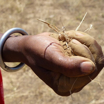
International Land Coalition Rangelands Initiative: Making rangelands secure

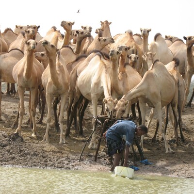
ACTIVE Feb 2028

Emerging public health threats in africa’s drylands.

• Burkina Faso
• Explore our work in the countries
• ILRI in the media

Policies and Design Processes to Enable Transformation

• Pereira, Laura
• Vrettos, Chris
• Cramer, Laura K.
• Drimie, Scott
• Muiderman, Karlijn
• Schapendonk, Frans
• Stringer, Lindsay C.
• Veeger, Marieke
• Vervoort, Joost M.
• Wamukoya, George

Opportunities to quantify resilience of dairy cattle to environmental stressors in Sub-Saharan Africa

• Oloo, Richard Dooso
• Ekine-Dzivenu, Chinyere C.
• Ojango, Julie M.K.
• Gebreyohanes, Gebregziabher
• Mrode, Raphael A.
• Okeyo Mwai, Ally
• Chagunda, Mizeck G.G.
• Publications
• Journal articles
• Presentations
• Infographics
• Browse archive

Climate-Smart Agriculture Practices for Mitigating Greenhouse Gas Emissions

Agricultural lands make up approximately 37% of the global land surface, and agriculture is a significant source of greenhouse gas (GHG) emissions, including carbon dioxide (CO 2 ), methane (CH 4 ) and nitrous oxide (N 2 O). Those GHGs are responsible for the majority of the anthropogenic global warming effect. Agricultural GHG emissions are associated with agricultural soil management (e.g. tillage), use of both synthetic and organic fertilisers, livestock management, burning of fossil fuel for agricultural operations, and burning of agricultural residues and land use change. When natural ecosystems such as grasslands are converted to agricultural production, 20–40% of the soil organic carbon (SOC) is lost over time, following cultivation. We thus need to develop management practices that can maintain or even increase SOCstorage in and reduce GHG emissions from agricultural ecosystems. We need to design systematic approaches and agricultural strategies that can ensure sustainable food production under predicted climate change scenarios, approaches that are being called climate‐smart agriculture (CSA). Climate‐smart agricultural management practices, including conservation tillage, use of cover crops and biochar application to agricultural fields, and strategic application of synthetic and organic fertilisers have been considered a way to reduce GHG emission from agriculture. Agricultural management practices can be improved to decreasing disturbance to the soil by decreasing the frequency and extent of cultivation as a way to minimise soil C loss and/or to increase soil C storage. Fertiliser nitrogen (N) use efficiency can be improved to reduce fertilizer N application and N loss. Management measures can also be taken to minimise agricultural biomass burning. This chapter reviews the current literature on CSA practices that are available to reduce GHG emissions and increase soil Csequestration and develops a guideline on best management practices to reduce GHG emissions, increase C sequestration, and enhance crop productivity in agricultural production systems.

• Kleineidam, K.
• Berendt, J.
• Bracken, C.
• Butterbach-Bahl, Klaus
• Chang, S.X.
• Reis Martins, M. dos
• Eckhardt, C.
• Fiedler, S.
• Goopy, John P.
• Görres, C.M.
• Hofmann, M.E.G.
• Jahangir, M.M.R.
• Jansen-Willems, A.
• Lenhart, K.
• Lewicka-Szczebak, D.
• Merbold, Lutz
• Molstad, L.
• Sanz-Cobena, A.
• Urquiaga, S.
• Wrage-Mönnig, N.
• Müller, Christoph
• GHG emissions

Related Publications

Greenhouse gas emissions from sheep excreta deposited onto tropical pastures in Kenya

• Oduor, Collins
• Gakige, Jesse K.
• Mwangi, Paul
• Leitner, Sonja

Health and socio-economic impacts of methane mitigation farm-scale digesters—Case study Ethiopia

• Mulat, Daniel

Exploring the role of seasonal variation in livestock feed composition on diet quality and methane emissions in Kenyan livestock

• Mutua, John
• Duncan, Alan J.
• Fraval, Simon
• Robinson, Timothy P.
• Notenbaert, An Maria Omer
• Watmough, Gary

Five key takeaways on livestock mitigation from the 2023 IPCC report on climate change

• Costa, Ciniro
• Arango, Jacobo
• Rosenstock, Todd S.
• Ferrari, Mireille
• Flintan, Fiona E.

Multiple mitigation strategies can lead to GHG emissions reduction in Kenyan dairy systems

• Graham, Michael
• Arndt, Claudia
• González-Quintero, Ricardo
• Korir, Daniel
• Ndung’u, Phyllis
• Özkan, Seyda
• Mottet, Anne

Effective Strategies to Mitigate Methane Emissions by Ruminants

Reducing agriculture emissions through improved farming practices

The agriculture sector’s role in greenhouse gas (GHG) emissions is widely known but not well understood. In truth, more than one-quarter of the world’s GHG emissions come from agriculture, forestry, and land-use change. And unless actively addressed, these emissions are likely to increase as more people populate the Earth and the need for food continues to grow. Our latest report, Agriculture and climate change , looks more deeply at these issues.

Global Warming of 1.5°C , the 2018 report by the Intergovernmental Panel on Climate Change (IPCC), makes clear that a “rapid and far-reaching” transition is required to limit the impact of climate change to 1.5 degrees Celsius. 1 Special report: Global warming of 1.5°C , the Intergovernmental Panel on Climate Change, 2018, ipcc.ch. Doing so would require staying within the cumulative carbon budget of 570 gigatons of equivalent carbon dioxide (GtCO 2 e), 2 For a two-thirds chance of limiting global mean surface temperature to 1.5°C above preindustrial levels. reaching net-zero carbon dioxide emissions globally around 2050, and significantly reducing the emissions of other gasses—including methane and nitrous oxide. Any successful scenario would mean major changes for agriculture, from how we farm, to how we eat and waste food, to how we manage our forests and natural carbon sinks.

Achieving these major changes may be more challenging for agriculture than for other sectors. Although the pace of emissions reduction remains too slow across the board, other sectors have identified many of the technologies that could substantially reduce emissions: these options don’t necessarily exist in agriculture. Agriculture is also significantly less consolidated than other sectors; reducing emissions requires action by one-quarter of the global population. Finally, the agriculture sector has a complicated set of objectives to consider alongside climate goals, including biodiversity, nutrition need, food security, and the livelihood of farmers and farming communities.

The first step in reducing emissions from agriculture is to produce food as efficiently as possible—that is, to change how we farm. A set of proven GHG-efficient farming technologies and practices—some of which are already being deployed—could achieve about 20 percent of the sector’s required emissions reduction by 2050.

Greenhouse gas–efficient farming practices: The global agriculture marginal abatement cost curve

Building on more than a decade of analysis of GHG abatement, we have identified the top 25 measures to reduce on-farm emissions and organized them into a marginal abatement cost curve (MACC). 3 For more on GHG abatement cost curves, see “ Greenhouse gas abatement cost curves .” These measures have the potential to abate up to a combined 4.6 GtCO 2 e 4 Calculated using 20-year global warming potential (GWP). For the purposes of policy discussion and target-setting, greenhouse gases are generally measured by global warming potential (GWP), a measure of how much energy the emissions of one ton of a gas will absorb over a given period, relative to the emissions of one ton of carbon dioxide. Given the importance of action and the short-term-gain potential of reducing agriculture’s methane emissions, our primary analysis is based on 20-year GWP values. For more information, see “Understanding global warming potentials,” EPA, epa.gov. by 2050 compared with business-as-usual emissions—a reduction of about 20 percent of total emissions from agriculture, forestry, and land use change. Moreover, the top 15 measures by abatement potential would contribute 85 percent of this emissions abatement and touch four major categories: energy, animal protein, crops, and rice cultivation.

For each measure, a bottom-up assessment of mitigation potential and cost was calculated using a synthesis of available literature; comparison across models of the Global Biosphere Management Model, Common Agricultural Policy Regionalised Impact, and Netherlands Environmental Agency; and discussions with relevant experts and practitioners. Costs shown include capital expenses, operating expenses, and potential cost savings. For all measures, the level of uptake and implementation was assessed to be as ambitious as possible while also being aware of the potential economic and noneconomic barriers to implement across regions, farm scales, and production systems. The interactive below illustrates some of these measures.

This analysis is distinctive in both its breadth and depth; our goal is to provide concrete guidance for policy makers, agriculture players, and academics alike to spur the necessary change in the agriculture sector. Some limitations of the global agriculture MACC should be noted:

• Costs shown are a weighted average and cannot therefore be assumed to apply in all regions.
• Potential overlap is controlled for through constrained adoption at a region and species level as well as limiting the MACC to measures that could feasibly be applied together.
• The MACC could substantially change over the next 30 years because of an increase in both measures and implementation rates.

In the course of human history, agriculture has responded to humanity’s greatest challenges. The sector has increased food production to a level that many believed impossible. The sector now has an opportunity to make yet another major contribution to humanity’s success during this crucial window for action.

Download the full report on which this article is based, Agriculture and climate change   (PDF–38MB).

Daniel Aminetzah is a senior partner in McKinsey’s New York office; Nicolas Denis is a partner in the Brussels office; Kimberly Henderson is a partner in the Washington, DC, office; Joshua Katz is a partner in the Stamford office; and Peter Mannion is a consultant in the Dublin office.

The authors wish to thank Justin Ahmed, Elaine Almeida, and Hannah Kitchel for their contributions to the full report.

Explore a career with us

Related articles.

Climate math: What a 1.5-degree pathway would take

Addressing climate change in a post-pandemic world

How to incentivize food systems to meet the realities of the 21st century

Introducing Drawdown Food – a new strategy for engaging agriculture in solving climate change

Project drawdown’s latest initiative will advance science and share insights at the intersection of food, agriculture, land use, and climate change..

Share this Story

Related topics, press contacts.

If you are a journalist and would like to republish Project Drawdown content, please contact [email protected] .

When we think of the causes of climate change, the first thing that comes to mind is often fossil fuel use for electricity production, transportation, or industry.

At the same time, an equally significant, yet far less recognized, contributor to climate change often gets short shrift: the global food system. A whopping 22–33% of all greenhouse gas emissions come from food, agriculture, and land (and ocean) use. 

Breakdown of global greenhouse gas emissions by sector and activity.  Data: Minx et al. (2021) and IPCC Sixth Assessment Report , Working Group Three

The systems we use to feed humanity have created a huge problem for Earth’s climate. But they also offer a huge opportunity to help halt climate change. 

“Using available technologies and practices, we can meet every person’s food needs while also neutralizing the food system’s impact on climate,” says Project Drawdown executive director Jonathan Foley, Ph.D., who is leading the initiative. “We just need to apply the right combinations of solutions in the right place at the right time.”

To that end, Project Drawdown is launching  Drawdown Food , a major new initiative to reduce the food system’s contribution to climate change. The initiative will lead research to define and refine best practices for enhancing global food security while minimizing adverse climate impacts. And it will apply that research to provide actionable information on ways movers and shakers can downsize greenhouse gas emissions from food and agriculture and make the most of the land’s capacity to draw carbon dioxide out of the atmosphere – based on timing, location, ancillary benefits, and more. 

The food system offers opportunities to reduce greenhouse gas concentrations in the atmosphere in two main ways. Most of the potential lies in cutting emissions. Additional gains come from removing carbon from the air by restoring ecosystems and enhancing soil health.

Alta Futures and the ZG Foundation are providing broad support for Drawdown Food’s analyses to better understand the food sector’s contributions to climate change and how food sector solutions can best be deployed to reduce this contribution. Funding from the Global Methane Hub will allow the Drawdown Food team to identify and deploy strategies to reduce methane emissions in food, agriculture, and land use. And the Asia Philanthropy Circle is underwriting work specific to Southeast Asia.  

In the weeks and months ahead, you’ll find regular reports on research-based intelligence at  Drawdown Food , here at Drawdown Insights, and shared through webinars, presentations, and research publications. Corporations, impact funders, and philanthropists will have opportunities to tap into the growing knowledge base and use it to maximize the impact of their climate efforts.

Most of all, the knowledge generated and shared will show the way to a food system that is healthier, not just for the climate and other planetary systems, but for all of humanity. 

We invite and encourage you to join us on this journey. Keep up to date by  subscribing to our biweekly newsletter and following us on social media.

More Insights

Sign Up For Our Newsletter

Loading metrics

Open Access

Peer-reviewed

Research Article

Rapid global phaseout of animal agriculture has the potential to stabilize greenhouse gas levels for 30 years and offset 68 percent of CO 2 emissions this century

Roles Conceptualization, Data curation, Formal analysis, Investigation, Methodology, Software, Visualization, Writing – original draft, Writing – review & editing

* E-mail: [email protected] (MBE); [email protected] (POB)

Affiliation Department of Molecular and Cell Biology, Department of Integrative Biology, Howard Hughes Medical Institute, University of California, Berkeley, CA, United States of America

Roles Conceptualization, Formal analysis, Writing – original draft, Writing – review & editing

Affiliations Department of Biochemistry (Emeritus), Stanford University School of Medicine, Stanford, CA, United States of America, Impossible Foods, Redwood City, CA, United States of America

• Michael B. Eisen, 
• Patrick O. Brown

• Published: February 1, 2022
• https://doi.org/10.1371/journal.pclm.0000010
• See the preprint
• Peer Review
• Reader Comments

Animal agriculture contributes significantly to global warming through ongoing emissions of the potent greenhouse gases methane and nitrous oxide, and displacement of biomass carbon on the land used to support livestock. However, because estimates of the magnitude of the effect of ending animal agriculture often focus on only one factor, the full potential benefit of a more radical change remains underappreciated. Here we quantify the full “climate opportunity cost” of current global livestock production, by modeling the combined, long-term effects of emission reductions and biomass recovery that would be unlocked by a phaseout of animal agriculture. We show that, even in the absence of any other emission reductions, persistent drops in atmospheric methane and nitrous oxide levels, and slower carbon dioxide accumulation, following a phaseout of livestock production would, through the end of the century, have the same cumulative effect on the warming potential of the atmosphere as a 25 gigaton per year reduction in anthropogenic CO 2 emissions, providing half of the net emission reductions necessary to limit warming to 2°C. The magnitude and rapidity of these potential effects should place the reduction or elimination of animal agriculture at the forefront of strategies for averting disastrous climate change.

Citation: Eisen MB, Brown PO (2022) Rapid global phaseout of animal agriculture has the potential to stabilize greenhouse gas levels for 30 years and offset 68 percent of CO 2 emissions this century. PLOS Clim 1(2): e0000010. https://doi.org/10.1371/journal.pclm.0000010

Editor: Ana Maria Loboguerrero, Alliance of Bioversity International and CIAT: Alliance of Bioversity International and International Center for Tropical Agriculture, COLOMBIA

Received: July 18, 2021; Accepted: November 29, 2021; Published: February 1, 2022

Copyright: © 2022 Eisen, Brown. This is an open access article distributed under the terms of the Creative Commons Attribution License , which permits unrestricted use, distribution, and reproduction in any medium, provided the original author and source are credited.

Data Availability: All code and data are available at https://github.com/mbeisen/LivestockClimateImpact .

Funding: There was no formal funding of this work. Michael Eisen is an Investigator with the Howard Hughes Medical Institute which funds all work in his lab. Patrick Brown is CEO of Impossible Foods, Inc.

Competing interests: We have read the journal’s policy and the authors of this manuscript have the following competing interests: Patrick Brown is the founder and CEO of Impossible Foods, a company developing alternatives to animals in food-production. Michael Eisen is an advisor to Impossible Foods. Both are shareholders in the company and thus stand to benefit financially from reduction of animal agriculture. Michael Eisen and Patrick Brown are co-founders and former members of the Board of Directors of the Public Library of Science.

Introduction

The use of animals as a food-production technology has well-recognized negative impacts on our climate. The historical reduction in terrestrial biomass as native ecosystems were transformed to support grazing livestock and the cultivation of feed and forage crops accounts for as much as a third of all anthropogenic CO 2 emissions to date [ 1 , 2 ]. Livestock, especially large ruminants, and their supply chains, also contribute significantly to anthropogenic emissions of the potent greenhouse gases (GHGs) methane and nitrous oxide [ 3 – 5 ].

Solving the climate crisis requires massive cuts to GHG emissions from transportation and energy production. But even in the context of large-scale reduction in emissions from other sources, major cuts in food-linked emissions are likely necessary by 2075 to limit global warming to 1.5°C [ 6 ]. While a reduction of food-linked emissions can likely be achieved by increasing agricultural efficiency, reducing food waste, limiting excess consumption, increasing yields, and reducing the emission intensity of livestock production [ 7 – 12 ], they are not anticipated to have the same impact as a global transition to a plant-rich diet [ 5 , 6 ].

Nutritionally balanced plant-dominated diets are common, healthy and diverse [ 13 – 17 ], but are rarely considered in comprehensive strategies to mitigate climate change [ 18 ], and there is controversy about their viability and the magnitude of their climate benefit [ 19 ]. One source of this discordance is that widely cited estimates of livestock contributions to global warming [ 4 , 5 , 20 ] account only for ongoing emissions, and not for the substantial and reversible warming impact of historical land use change [ 1 , 21 ].

The Food and Agriculture Organization (FAO) of the United Nations estimates that emissions from animal agriculture represent around 7.1 Gt CO 2 eq per year [ 5 ], 14.5% of annual anthropogenic greenhouse gas emissions, although this is based on outdated data and likely now represents and underestimate [ 20 ], and recent estimates [ 1 ] suggest that on the order of 800 Gt CO 2 equivalent carbon could be fixed via photosynthesis if native biomass were allowed to recover on the 30% of Earth’s land surface current devoted to livestock production. Thus, crudely, eliminating animal agriculture has the potential to reduce net emissions by the equivalent of around 1,350 Gt CO 2 this century. To put this number in perspective, total anthropogenic CO 2 emissions since industrialization are estimated to be around 1,650 Gt [ 2 ].

However, a substantial fraction of the emissions impact of animal agriculture comes from methane (CH 4 ) and nitrous oxide (N 2 O), which decay far more rapidly than CO 2 (the half-lives of CH 4 and N 2 O are around 9 and 115 years, respectively), and recent studies have highlighted the need to consider these atmospheric dynamics when assessing their impact [ 22 – 24 ]. Of critical importance, many of the beneficial effects on greenhouse gas levels of eliminating livestock would accrue rapidly, via biomass recovery and decay of short-lived atmospheric CH 4 , and their cooling influence would be felt for an extended period of time.

Our goal here was to accurately quantify the full impact of current animal agriculture on the climate, taking into account the currently unrealized opportunities for emission reduction and biomass recovery together, and explicitly considering the impact of their kinetics on warming. Our approach differs from other recent studies [ 25 , 26 ] in that we did not attempt to predict how global food production and consumption might change with growing populations, economic development, advances in agriculture, climate change and other socioeconomic factors. Nor do we tackle the social, economic, nutrition and agricultural challenges inherent to such a large change in global production.

We used publicly available, systematic data on livestock production in 2019 [ 27 ], livestock-linked emissions [ 3 , 27 ], and biomass recovery potential on land currently used to support livestock [ 1 ] to predict how the phaseout of all or parts of global animal agriculture production would alter net anthropogenic emissions. We then used a simple climate model to project how these changes would impact the evolution of atmospheric GHG levels and warming for the rest of the century.

We calculated the combined impact of reduced emissions and biomass recovery by comparing the cumulative reduction, relative to current emission levels, of the global warming potential of GHGs in the atmosphere for the remainder of the 21st century under different livestock replacement scenarios to those that would be achieved by constant annual reductions in CO 2 emissions.

Modeling the effect of eliminating animal agriculture on GHG levels

We implemented a simple climate model that projects atmospheric GHG levels from 2020 to 2100 based on a time series of annual emissions of CO 2 , CH 4 and N 2 O and a limited set of parameters. We then compared various hypothetical dietary perturbations to a “business as usual” (BAU) reference in which emissions remain fixed at 2019 levels, based on global emissions data from FAOSTAT [ 27 ].

The dietary scenarios include the immediate replacement of all animal agriculture with a plant-only diet (IMM-POD), a more gradual transition, over a period of 15 years, to a plant-only diet (PHASE-POD), and versions of each where only specific animal products were replaced.

We updated estimates of global emissions from animal agriculture using country-, species- and product-specific emission intensities from the Global Livestock Environmental Assessment Model [ 3 ], and country-specific data on primary production of livestock products from the Food and Agriculture Organization (FAO) database FAOSTAT [ 27 ].

Based on this analysis, in 2019 (the most recent year for which full data are available), global production of animal-derived foods led to direct emissions of 1.6 Gt CO 2 , due primarily to energy use (as our model assumes constant overall rates of consumption, we excluded emissions due to land clearing, which are associated with agricultural expansion), 120 Mt CH 4 due primarily to enteric fermentation and manure management, and 7.0 Mt N 2 O due primarily to fertilization of feed crops and manure management ( Fig 1 and S1 Fig ).

• PPT PowerPoint slide
• PNG larger image
• TIFF original image

Total CO 2 equivalent emissions (A) assembled from species, product and country-specific production data from FAOSTAT for 2019 and species, product, region and greenhouse-gas specific emissions data from GLEAM [ 3 ], using CO 2 equivalents of 34 for CH 4 and 298 for N 2 O. Land use (B) assembled from species, product and country-specific production data from FAOSTAT for 2019 and species and product specific land use data from [ 12 ].

https://doi.org/10.1371/journal.pclm.0000010.g001

These numbers are broadly consistent with other recent estimates [ 4 , 5 , 26 ], and correspond, respectively, to 4% of CO 2 , 35% of CH 4 and 66% of N 2 O emissions from all human activities, using total human emissions data from FAOSTAT [ 27 ]. Combining the effects of the three gases, using global warming potentials from [ 28 ], results in 6.3 Gt CO 2 eq, with the major difference from the 7.1 Gt CO 2 eq number cited above coming from our exclusion of ongoing land use change.

We modeled the recovery of biomass on land currently used in livestock production using data from [ 1 ] who estimate that the return of land currently used in livestock production to its native state would sequester, over 30 years, 215.5 Gt of carbon (equivalent to 790 Gt of CO 2 ) in plant and non-living biomass. A similar estimate was obtained by [ 21 ].

We assumed in all these hypothetical scenarios that non-agricultural emissions would remain constant; that food from livestock is replaced by a diverse plant based diet; and that, when land is removed from livestock production, the conversion of atmospheric CO 2 into terrestrial biomass occurs linearly over the subsequent thirty years. (We consider alternative assumptions in the “Sensitivity Analysis” section below).

We emphasize that we are not predicting what will happen to global diets. Rather we are projecting simplified scenarios of dietary change forward through time to characterize and quantify the climate impact of current animal agriculture production. Our climate model is intentionally simple, considering only the partition of terrestrial emissions into the atmosphere, and the decay of methane and nitrous oxide, although it replicates the qualitative behavior of widely used MAGICC6 [ 29 ].

Fig 2 shows annual emissions and projected atmospheric levels of CO 2 , CH 4 and N 2 O under BAU and PHASE-POD through the end of the century (projections for IMM-POD and additional scenarios are shown in S2 – S32 Figs).

(A) Projected annual emissions of CO 2 , CH 4 and N 2 O for Business as Usual (red) and PHASEPOD (green) assuming a 15 year transition to new diet and 30 year carbon recovery. (B) Projected atmospheric concentrations of CO 2 , CH 4 and N 2 O under each emission scenario.

https://doi.org/10.1371/journal.pclm.0000010.g002

Rapid phaseout of animal agriculture would freeze increases in the warming potential of the atmosphere for 30 years

The impact of PHASE-POD on CO 2 emissions would be greatest in the period between 2030 and 2060, when biomass recovery on land previously occupied by livestock or feed crops reaches its peak, slowing the rise of atmospheric CO 2 levels during this interval.

Atmospheric CH 4 and N 2 O levels continue to increase in both BAU and PHASE-POD during the transition period, but begin to drop in PHASE-POD as the abatement of animal agriculture-linked emissions accelerates. CH 4 , with a half-life in the atmosphere of around 9 years, approaches a new and lower steady-state level towards the end of the century, while N 2 O, with a half-life of around 115 years, does so over a longer time-scale.

To capture the combined global warming impact of the changing levels of these GHGs, we calculated radiative forcing (RF), the reduction in radiative cooling by GHG absorption of infrared radiation, using the formulae described in [ 30 , 31 ] and used in MAGICC6 [ 29 ].

Fig 3 shows that with PHASE-POD there would effectively be no net increase in RF between 2030 and 2060. And even after that 30-year pause in the previously monotonically increasing global warming potential of the atmosphere, the difference in RF between the POD and BAU scenarios would continue to increase, due to the absence of direct emissions from animal agriculture and the continuing decay of previously emitted CH 4 and N 2 O towards lower steady-state values.

Effect of eliminating emissions linked to animal agriculture and of biomass recovery on land currently used in animal agriculture on Radiative Forcing (RF), a measure of the instantaneous warming potential of the atmosphere. RF values computed from atmospheric concentrations in by formula of [ 30 , 32 ] as modified in MAGICC6 [ 29 ] with adjustment for gases other than CO 2 , CH 4 and N 2 O as described in text.

https://doi.org/10.1371/journal.pclm.0000010.g003

Rapid phaseout of animal agriculture could achieve half of the emission reductions needed to meet Paris Agreement GHG targets

By the end of the century the RF under PHASE-POD would be 3.8 Wm -2 compared to 4.9 Wm -2 for BAU, a reduction in RF equivalent to what would be achieved by eliminating 1,680 Gt of CO 2 emissions ( S33 Fig ), or 46 years of global anthropogenic CO 2 emissions at the current rate of 36 Gt/year.

In 2010, the climate modeling community defined a series of four “Representative Concentration Pathways” that capture a wide range of future warming scenarios, leading to 2100 RF levels of 8.5, 6.0, 4.5 and 2.6 Wm -2 (which is approximately the RF of current atmospheric greenhouse gas levels), respectively [ 33 , 34 ]. These model pathways were extended after the Paris Agreement to include a target of 1.9 Wm -2 . Although the exact relationship between RF and global warming is incompletely understood, 2100 RF values of 1.9 and 2.6 Wm -2 are generally used as targets for limiting warming in this century to 1.5˚C and 2.0˚C, respectively, over the baseline pre-industrial global average temperature [ 18 ].

Reducing 2100 RF from 4.9 Wm -2 under BAU to 2.6 Wm -2 would require a reduction of atmospheric CO 2 levels by 204 ppm, equivalent to 3,230 Gt of CO 2 emissions ( Fig 4 and S33 Fig ), and an additional 47 ppm reduction, equivalent to 750 Gt of CO 2 emissions, would be required to reach 1.9 Wm -2 .

Using projected CH 4 and N 2 O levels in 2100 under business as usual diet as a baseline for RF calculation, we computed the CO 2 reductions necessary to reduce RF from the business as usual diet level of RF = 1.31 to the bovid-free diet level of RF = 4.09 (1300 Gt CO 2 ), the plant-only diet level of RF = 3.83 (1680 Gt CO 2 ), the 2.0° C global warming target of RF = 2.6 (3230 Gt CO 2 ) and the 1.5° C global warming target of RF = 1.9 (3980 Gt CO 2 ). For this analysis we used a corrected RF that accounts for the absence of other gases in our calculation by training a linear regression model on published MAGICC6 output to estimate from CO 2 , CH 4 and N 2 O levels the residual RF impact of other gases.

https://doi.org/10.1371/journal.pclm.0000010.g004

Thus the 1,680 Gt of CO 2 equivalent emissions reductions from the phased elimination of animal agriculture, would, without any other intervention to reduce GHG emissions, achieve 52% of the net GHG emissions reductions necessary to reach the 2100 RF target of 2.6 Wm -2 and 42% of the emissions reductions necessary to reach the 1.9 Wm -2 target [ 18 ].

Eliminating animal agriculture has the potential to offset 68 percent of current anthropogenic CO 2 emissions

While widely used, such single point estimates of radiative forcing tell an incomplete story, as temperature change, and other climate impacts, depend cumulatively on the temporal trajectories of changing atmospheric greenhouse gas levels.

To capture such dynamic effects, we computed, for each dietary scenario, the integral with respect to time of the RF difference between the scenario and BAU, from 2021 (the start of the intervention in this model) to a given year “y”. We designate this cumulative RF difference for year y , CRFD y . We then determined, for each dietary scenario and year y , what level of reduction in annual CO 2 emissions alone, relative to BAU, would yield the same CRFD y , and designate this annual CO 2 equivalent aCO 2 eq y (see S36 and S37 Figs for details of these equivalences).

Critical features of aCO 2 eq are that it operates directly on RF inferred from combined trajectories of atmospheric levels of all GHGs, and thus can directly capture the effects of arbitrarily complex interventions, and that it equates the cumulative RF impact of an intervention over a specified time window to a single number: the sustained reductions in CO 2 emissions that would have the same cumulative impact.

aCO 2 eq is closely related to, and motivated by similar goals as, CO 2 -forcing-equivalent (CO 2 -fe) emissions [ 35 ], which equates an arbitrary emission trajectory of all GHGs to a trajectory of CO 2 emissions that would produce the same trajectory of RF, and GWP* [ 22 – 24 ], which uses various formulae to equate changes in GHG emissions to instantaneous CO 2 pulses.

Fig 5 shows the aCO 2 eq for different scenarios for reference years 2050 (to capture short term impacts) and 2100 ( S38 Fig shows the full dependence of aCO 2 eq on the reference year). The aCO 2 eq 2100 for PHASE-POD is -24.8 Gt/year. As global anthropogenic CO 2 emissions are currently approximately 36 Gt/year, that PHASE-POD would have the same effect, through the end of the century, as a 68% reduction of CO 2 emissions.

Bars show sustained reduction in annual CO 2 emissions necessary to equal cumulative reduction in radiative forcing of the given scenario in 2050 (blue) and 2100 (orange).

https://doi.org/10.1371/journal.pclm.0000010.g005

Replacing ruminants achieves over 90 percent of climate benefit of eliminating animal agriculture

We next computed aCO 2 eq 2100 for the 15 year phaseout of individual animal products and product categories (Figs 5 and 6A ; Table 1 ), using the species- and product-specific emissions and land use values described above. Beef alone accounts for 47% of the benefits of phasing out all animal agriculture, and cow milk 24%. Meat and milk from bovids (cattle and buffalo) account for 79% of the climate opportunity. Although they provide less than 19% of the protein in the human diet [ 27 ], ruminants (cattle, buffalo, sheep and goats) collectively account for 90% of the aCO 2 eq 2100 of all livestock.

(A) Total annualized CO 2 equivalents through 2100, aCO 2 eq 2100 , for all tracked animal products, and Emission Intensities based on aCO 2 eq 2100 on a per unit production (B) or per unit protein (C) basis. For (B) and (C) we also convert the values to driving equivalents using a value of 0.254 kg CO 2 eq per km driven of an internal combustion engine fueled sedan in the United States from life cycle analyses described in [ 36 ].

https://doi.org/10.1371/journal.pclm.0000010.g006

https://doi.org/10.1371/journal.pclm.0000010.t001

These product-specific aCO 2 eq’s can be interpreted on a per product unit ( Fig 6B ) or per protein unit ( Fig 6C ) as emissions intensities. Eliminating the consumption of a kilogram of beef, for example, is equivalent to an emissions reduction of 297 kg CO 2 . 38% (113 kg aCO 2 eq) comes from reduced emission, in line with the mean estimate of 99.5 kg CO 2 eq from a systematic meta analysis of GHG emissions from agricultural products [ 12 ], with the remaining 62% from biomass recovery.

As with the total numbers, ruminant meat has the largest emissions intensities, per unit (289 kg CO 2 eq per kg consumer product) and per protein (1,279 kg CO 2 eq per kg protein). The most efficient animal products on a per protein basis are chicken meat (56 kg CO 2 eq per kg protein) and eggs (49 kg CO 2 eq per kg protein), roughly 25 times lower than per protein emissions intensities for ruminant meat.

To connect these numbers to other sources of GHGs, we converted these emissions intensities to distances one would have to drive a typical 2021 model gas-fueled passenger car to produce the same emissions, based on a full life-cycle analysis of auto emissions [ 36 ] ( Fig 6B and 6C ). One kg of beef, for example, has the same emissions impact as driving 1,172 km in a typical US car (or 339 miles per pound).

Sensitivity to assumptions

Our default model assumes a gradual phaseout of animal agriculture over a period of 15 years, producing an aCO 2 eq 2100 of -24.8 Gt/year. If we assume immediate elimination ( S2 Fig ), the aCO 2 eq 2100 is -28.3 Gt/year ( Fig 7A ), a 14% increase in magnitude of the effect. If we assume a phaseout over 30 years ( S3 Fig ), the aCO 2 eq 2100 is -21.3 Gt/year ( Fig 7A ), a 14% reduction.

The grey line in each plot is PHASE-POD, the default scenario of 15 year phaseout, 30 year carbon recovery, livestock emissions from FAOSTAT, and a diverse plant replacement diet based on [ 26 ]. (A) Effect of the immediate elimination of animal agriculture (red line) or a slower, 30 year, phaseout (blue line). (B) Effect of slower carbon recovery reaching completion after 50 years (red line) or 70 years (blue line). (C) Effect of using high (green line) or low (red line) estimates of above ground carbon recovery from [ 1 ]. (D) Effect of reducing either the efficiency or extent of carbon recovery.

https://doi.org/10.1371/journal.pclm.0000010.g007

Our default model also assumes that biomass will recover linearly over 30 years, following [ 1 ], but there is considerable uncertainty in the literature, with estimates ranging from 25 to 70 years [ 37 – 39 ]. If we assume recovery takes 50 years ( S4 Fig ), the aCO 2 eq 2100 is -22.4 Gt/year, and if it takes 70 years ( S5 Fig ), the aCO 2 eq 2100 is -20.1 Gt/year, or reductions of 10% and 19% respectively ( Fig 7B ). We also note that passive recovery is not the only option. Further research is required to define optimal management practices for recovery of ecosystems currently impacted by animal agriculture and to estimate the rate and magnitude of their potential impact on climate. But there is evidence that deliberate, active management of ecosystem recovery to optimize for carbon sequestration could accelerate and increase the magnitude of carbon storage on land transitioning from intensive agricultural use [ 40 ].

Estimates of the biomass recovery potential of land currently used for animal agriculture have a high degree of uncertainty. Using the low estimate ( S6 Fig ) of [ 1 ], which addresses uncertainty in above-ground biomass yields an aCO 2 eq 2100 of -21.2 Gt/year ( Fig 7C ), a 14% reduction in magnitude relative to the median value from [ 1 ]. Using the high estimate ( S7 Fig ) of [ 1 ] yields an aCO 2 eq 2100 of -28.1 Gt/year ( Fig 7C ), an increase in magnitude of 13% increase.

A major area of uncertainty not addressed by [ 1 ] is the extent to which the carbon recovery potential of land that transitions away from use in animal agriculture would be realized in the face of other land use pressures. The land needed to replace animal derived foods in the global diet is accounted for in [ 1 ], but not other potential large-scale non-food uses such as biofuel production. While it is beyond the scope of this work to model these uses explicitly, Fig 7D shows the expected RF trajectories if we assume reduced recovery fractions of 25% ( S8 Fig ), 50% ( S9 Fig ), 75% ( S10 Fig ) and 100% ( S11 Fig ), which yield aCO 2 eq 2100 of -21.6, -18.3, -15.0, and -11.6 Gt/year respectively, highlighting the importance of carbon recovery in realizing the climate potential of ending animal agriculture. It is important to note that there is substantial variance in the biomass potential between regions and ecosystems, and recent modeling work by [ 21 ] indicates that half of the biomass recovery potential of land currently used for agriculture could be realized by restoration of 25% of the relevant land.

Our estimate of global emissions due to animal agriculture based on FAO data and analyses of 1.6 Gt CO 2 , 122 Mt CH 4 and 7.0 Mt N 2 O differ in key ways from recent estimates of [ 26 ] of 3.2 Gt CO 2 , 102 Mt CH 4 and 3.9 Mt N 2 O. Using these emissions estimates for livestock ( S12 Fig ) yields an aCO 2 eq 2100 of PHASE-POD of -23.6 Gt/year ( S40 Fig ), a 5% decrease in magnitude.

The models described above assume that the protein currently obtained from animal products would be replaced with a diverse plant based diet, scaled to replace animal products on a protein basis, and agriculture emissions data from FAOSTAT. We considered as an alternative emissions projected from a diverse plant based diet based on data from [ 26 ], scaled to replace animal products on a protein basis. This replacement diet ( S13 Fig ) yields an aCO 2 eq 2100 for PHASE-POD of animal agriculture of -23.7 Gt/year ( S40 Fig ), a 5% decrease in magnitude.

In some areas, the removal of land from use in animal agriculture may lead to an increase in wild ruminant population. Although this is difficult to model globally, this would offset some of the beneficial impacts of reductions in methane emissions from livestock [ 41 ].

This analysis only considered consumption of terrestrial animal products, neglecting emissions and land use (via feed production) associated with seafood capture and aquaculture. While the land and emissions impact of seafood consumption has received comparably little attention, several studies have pointed to at least 500 Mt of CO 2 equivalent emissions per year from seafood [ 12 , 42 , 43 ]. Recent work has also suggested that the disruption of carbon storage due to seafood harvesting via trawling repartitions from 0.58 up to 1.47 Gt CO 2 equivalent carbon per year from sediment into the water column, with the potential to drive atmospheric increases of similar magnitude [ 44 ].

Widely used climate models consider temporal and spatial variation in emissions; feedback between a changing climate and anthropogenic and natural emissions, carbon sequestration, atmospheric chemistry and warming potential; the impact of climate on human social, political and economic behavior. Ours does not. We ran our model on emissions data from the pathways described in [ 45 ] and compared our atmospheric level and RF outputs to theirs, and found them to be in broad qualitative agreement. Thus, while other models could provide more precise estimates, we do not believe they would alter our major conclusions.

Our analysis has provided a quantitative estimate of the potential climate impact of a hypothetical, radical global change in diet and agricultural systems. We have shown that the combined benefits of removing major global sources of CH 4 and N 2 O, and allowing biomass to recover on the vast areas of land currently used to raise and feed livestock, would be equivalent to a sustained reduction of 25 Gt/year of CO 2 emissions.

Crucially eliminating the use of animals as food technology would produce substantial negative emissions of all three major GHGs, a necessity, as even the complete replacement of fossil fuel combustion in energy production and transportation will no longer be enough to prevent warming of 1.5°C [ 6 – 8 ].

The transition away from animal agriculture will face many obstacles and create many challenges. Meat, dairy and eggs are a major component of global human diets [ 27 ], and the raising of livestock is integral to rural economies worldwide, with more than a billion people making all or part of their living from animal agriculture.

Although animal products currently provide, according to the most recent data from FAOSTAT, 18% of the calories, 40% of the protein and 45% of the fat in the human food supply, they are not necessary to feed the global population. Existing crops could replace the calories, protein and fat from animals with a vastly reduced land, water, GHG and biodiversity impact, requiring only minor adjustments to optimize nutrition [ 25 ].

The economic and social impacts of a global transition to a plant based diet would be acute in many regions and locales [ 46 ], a major obstacle to their adoption. It is likely that substantial global investment will be required to ensure that the people who currently make a living from animal agriculture do not suffer when it is reduced or replaced. And, while it is expected that the phaseout of animal agriculture would lead to global increases in food availability as edible crops cease to be diverted for animal feed [ 47 ], investment will also be required to prevent local food insecurity in regions where wide-scale access to a diverse and healthy plant-based diet is currently lacking and to ensure proper nutrition. But, in both cases, these investments must be compared to the economic and humanitarian disruptions of significant global warming [ 48 , 49 ].

Although, as discussed above, there are many uncertainties in our estimates, our assumption that “business as usual” means animal agriculture will continue at current levels was highly conservative, as rising incomes are driving ongoing growth in global animal product consumption [ 50 ]. It is estimated that global demand for animal based foods will increase by nearly 70 percent by 2050 [ 50 ]. For example, using land use data from [ 12 ] and consumption data from FAOSTAT, extending the current diet of wealthy industrialized countries (OECD) to the current global population would require an additional 35 million km 2 to support livestock production—an area roughly equal to the combined area of Africa and Australia.

While such an expansion may seem implausible, even partial destruction of Earth’s critical remaining native ecosystems would have catastrophic impacts not just on the climate, but on global biodiversity [ 51 – 53 ] and human health [ 13 , 21 , 54 – 58 ].

Given these realities, even with the many challenges that upending a trillion dollar a year business and transforming the diets of seven billion people presents, it is surprising that changes in food production and consumption are not at the forefront of proposed strategies for fighting climate change. Although all of the strategies presented as part of the recent Intergovernmental Panel on Climate Change (IPCC) report on steps needed to keep global warming below 1.5˚C [ 18 ] acknowledge the need for significant negative emissions, none propose even a reduction in per capita livestock consumption below current levels ( Fig 8 ).

We downloaded data for the Shared Socioeconomic Pathways (SSPs) [ 45 ] from the SSP database (Version 2.0; last updated December 2018), and plot here the inferred per capita livestock production for scenarios meant to reach an RF target of 1.9 in 2100. While there is widespread acknowledgement of the impact that ongoing animal agriculture has on the climate, it is notable that most of these scenarios, which represent the most aggressive proposed mitigation strategies in this modeling framework, anticipate an increase in per capita livestock consumption, and none anticipate any significant reduction below current levels, in contrast to the complete elimination we propose here.

https://doi.org/10.1371/journal.pclm.0000010.g008

Even if the negative emission technology the IPCC anticipates, BECCS (bio-energy combined with carbon capture and storage), proves to be viable at scale, it will require large amounts of land [ 59 ], and the only way to get that land without massive collateral damage is by displacing animal agriculture, primarily land-intensive ruminants. Thus, all potential solutions to the climate crisis likely require some form of large scale dietary change.

It is important to emphasize that, as great as the potential climate impact of ending animal agriculture may be, even if it occurred, and even if all of the benefits we anticipate were realized, it would not be enough on its own to prevent catastrophic global warming. Rather we have shown that global dietary change provides a powerful complement to the indispensable transition from fossil fuels to renewable energy systems. The challenge we face is not choosing which to pursue, but rather in determining how best to overcome the many social, economic and political challenges incumbent in implementing both as rapidly as possible.

Data and code availability

Analyses were carried out in Python using Jupyter notebooks. All data, analyses and results presented here are available at github.com/mbeisen/LivestockClimateImpact .

Updating estimates of emissions from animal agriculture

We obtained country, species, herd and product type specific CO 2 , CH 4 and N 2 O emission data for terrestrial livestock from the public version of GLEAM 2.0 [ 3 ] downloaded from http://www.fao.org/gleam/results/en/ . GLEAM contains data for cattle, buffalo, sheep, goats, pigs and chickens, and attributes emissions to meat, milk and eggs. Although GLEAM further breaks down emissions based on herd type and production system, we used aggregate data for all herds and production types in the country. We did not include CO 2 emissions linked to land-use change, as this is associated with increases in livestock production which are explicitly not considered by our model.

We obtained livestock production data for 2019 (the most recent year available) from the “Production_LivestockPrimary” datafile in FAOSTAT [ 27 ]. We extracted from Production_LivestockPrimary the amount (in tonnes), for all countries, of primary domestic production of meat from cattle, buffalo, sheep, goat, pig, chicken and duck, milk from cows, buffalo, sheep and goat, and eggs from poultry. We computed meat and protein yields from the carcass weight data reported by GLEAM.

We scaled the GLEAM emission data to current production data from FAOSTAT, using GLEAM data for entire herds based on carcass weight for meat, and production weight for milk and eggs. As GLEAM does not provide data for ducks, we used values for chicken. The scaling was done using country-specific livestock production data from FAOSTAT and regional data from GLEAM.

Estimating species-specific land use

We combined livestock production data with average species and product-specific land use data from [ 12 ] to estimate species, product and country-specific land use data associated with animal agriculture. We use data for cattle meat for buffalo meat, and cow milk for milk from buffalo, goat and sheep. The data are reported in m m 2 ( year )(100 g protein ) −1 except for milk which is reported in m 2 ( year )( liter ) −1 which we convert to m 2 ( year )( kg primary production ) −1 using conversion factors inferred from GLEAM, which reports both protein and primary production data.

The total land use for animal agriculture inferred from this analysis is 33.7 million km 2 , almost identical to the 33.2 million km 2 estimated by [ 1 ] from satellite imagery.

Emissions from agriculture

We used the Environment_Emissions_by_Sector_E_All_Data_(Normalized) data table from FAOSTAT, projecting from the most recent year of 2017 to 2019 by assuming that the average annual growth from 2000 to 2017 continued in 2018 and 2019.

Replacement diets

We modeled agricultural emissions under a business as usual (BAU) diet as remaining at 2019 levels. When modeling reductions in livestock consumption, we assumed protein from livestock products would be replaced with the equivalent amount of protein from current food crops, and used per unit protein emission intensities computed from FAOSTAT to infer emissions from this replacement diet. As an alternative we used emission intensities from [ 26 ] as described in the Sensitivity section. For diets involving the removal of one or more specific animal products, we scaled these dietary replacement emissions by the fraction of animal protein obtained from that product, and scaled biomass recovery by the fraction of animal agriculture land attributed to that product.

Replacement scenarios

We also include in the supplemental data a version of the analysis in which the hypothetical transition is instantaneous (IMM-POD).

We assume that, when animal-derived food consumption is reduced in a year by a fraction Δf , that carbon recovery on a corresponding fraction of land begins immediately and continues at a constant rate until it reaches 100% after 30 years [ 1 ] (see also Fig 7 for 50 and 70 year recovery timelines).

Converting between emissions and atmospheric concentrations of GHGs

The total mass of gas in the atmosphere is 5.136 * 10 21 g, at a mean molecular weight of 28.97 g/mole [ 60 ], or 1.77e+20 total moles of gas. Hence 1 ppb is 1.77*10 11 moles and 1 ppm is 1.77 * 10 14 moles.

Estimating global non-anthropomorphic emissions

Both CH 4 and N 2 O decay at appreciable rates, with half-lives of approximately 9 years for CH 4 [ 62 ] and 115 years for N 2 O [ 63 ], although these estimates are being continuously updated [ 64 ]. We balanced the corresponding decay equations against historical emissions and atmospheric levels, inferring unaccounted for and presumably non-anthropogenic sources leading to mole fraction equivalent increases of CH 4 of 25 ppb/year and N 2 O of 1.0 ppb/year.

Projections of atmospheric gas levels

Radiative forcing

We adopt the commonly used formula for radiative forcing (RF) which derives from [ 30 , 32 ] as modified in the climate modeling program MAGICC6 [ 29 ].

C 0 , M 0 and N 0 are the preindustrial levels of the corresponding gases.

Computing emissions and land carbon opportunity cost

The factor of 2 accounts for the half of CO 2 emissions that go to terrestrial sinks.

Computing carbon emissions budgets for RF 2.6 and 1.9

As the RF calculation used in MAGICC6 account for other gases and effects beyond the three gases used here, we used multivariate linear regression as implemented in the Python package scikit-learn to predict the complete RF output of MAGICC6 using data downloaded from the Shared Socioeconomic Pathways (SSPs) [ 45 ]. The model was trained on atmospheric concentrations of CO 2 , CH 4 and N 2 O to predict the difference between the MAGICC6 RF and the RF calculated using only CO 2 , CH 4 and N 2 O. Then, for timepoints in our scenarios we computed RF as above from CO 2 , CH 4 and N 2 O concentrations, and added to this the adjustment from the linear regression model. We use this RF in Figs 3 and 4 .

In the SSP file:

C = Diagnostics|MAGICC6|Concentration|CO 2

M = Diagnostics|MAGICC6|Concentration|CH 4

N = Diagnostics|MAGICC6|Concentration|N 2 O

MAGICC6 RF = Diagnostics|MAGICC6|Forcing

To compute aCO 2 eq y , the annual CO 2 equivalent emission change of each emissions scenario, we first ran scenarios in which annual CO 2 emissions were reduced from 50 Gt/year to 1 Gt/year in increments of 1 Gt/year, then from 1 Gt/year to 10 Mt/year in increments of 10 Mt/year, and then from 1 Mt/year to 100 kT/year in increments of 100 kT/year. For each of these calibration scenarios, and for all years y from 2021 to 2100, we computed the total RF difference between the calibration scenario and BAU, from 2021 to y .

For each multi-gas emissions scenario, we similarly computed CRFD y , and determined what constant level of reduction in annual CO 2 emissions alone by interpolation using the CRFD y of the calibration scenarios, and designate this annual CO 2 equivalent aCO 2 eq y .

Product equivalents

To compute per product unit and per protein emissions equivalents, we divided aCO 2 eq 2100 for immediate elimination of the product (in kg CO 2 eq/year) by the annual production of the product (in kg production/year) yielding a per product unit emission equivalent measured in kg CO 2 eq per kg production.

For example, assuming, as our model does, that emissions and land use scale with consumption, if annual beef production were reduced by one tonne (1,000 kg) per year, it would result in corresponding annual reductions of -3,476 kg CO 2 , -726 kg CH 4 and -36 kg N 2 O, and would initiate 30 year biomass recovery of 6,050,000 kg of CO 2 equivalent carbon on 25.2 ha of land.

The cumulative reduction in RF, through 2100, of such annual emissions reductions and biomass recovery would be equivalent to a CO 2 emission reduction of 199,000 kg/year. The ratio of these two rates, -199,000 kg CO 2 eq/year over 1,000 kg beef/year yields -199 kg CO 2 eq per kg beef as a measure of the warming impact of one kg of beef. Adjusting this for the dressing percentage of beef (the values reported by FAO, and used in these calculations, are carcass weight, of which only approximately ⅔ ends up as a consumer product) yields the values shown in Fig 6 .

For all meat products we scaled the production amount by a typical dressing percentage of ⅔ to convert to consumer product units. For protein unit equivalents we used protein yields from GLEAM. To convert to driving equivalents we used a value of .254 kg CO 2 eq per km driven taken from life cycle analyses reviewed in [ 36 ].

Supporting information

S1 fig. 15yr phaseout vs. elimination..

(A) Projected annual emissions of CO 2 , CH 4 and N 2 O for each scenario. (B) Projected atmospheric concentrations of CO 2 , CH 4 and N 2 O under each emission scenario. (C) Radiative Forcing (RF) inferred from atmospheric concentrations in (B) by formula of [ 30 , 32 ] as modified in MAGICC6 [ 29 ]. Only differences between PHASE-POD default assumptions (15yr phaseout, 30yr carbon recovery, 100% carbon recovery, BAU non-agriculture emissions, FAO crop replacement, and FAO animal ag emissions) are given.

https://doi.org/10.1371/journal.pclm.0000010.s001

S2 Fig. 15yr phaseout vs. elimination.

https://doi.org/10.1371/journal.pclm.0000010.s002

S3 Fig. 15yr vs. 30yr phaseout.

https://doi.org/10.1371/journal.pclm.0000010.s003

S4 Fig. 30yr vs. 50yr biomass recovery.

https://doi.org/10.1371/journal.pclm.0000010.s004

S5 Fig. 30yr vs. 70yr biomass recovery.

https://doi.org/10.1371/journal.pclm.0000010.s005

S6 Fig. Hayek median vs. low recovery potential.

https://doi.org/10.1371/journal.pclm.0000010.s006

S7 Fig. Hayek median vs. high recovery potential.

https://doi.org/10.1371/journal.pclm.0000010.s007

S8 Fig. 100% vs. 75% biomass recovery.

https://doi.org/10.1371/journal.pclm.0000010.s008

S9 Fig. 100% vs. 50% biomass recovery.

https://doi.org/10.1371/journal.pclm.0000010.s009

S10 Fig. 100% vs. 25% biomass recovery.

https://doi.org/10.1371/journal.pclm.0000010.s010

S11 Fig. 100% vs. 0% biomass recovery.

https://doi.org/10.1371/journal.pclm.0000010.s011

S12 Fig. FAO vs. Xu emissions.

https://doi.org/10.1371/journal.pclm.0000010.s012

S13 Fig. FAO vs. Xu replacement diet.

https://doi.org/10.1371/journal.pclm.0000010.s013

S14 Fig. 15yr phaseout vs. net zero CO 2 .

https://doi.org/10.1371/journal.pclm.0000010.s014

S15 Fig. Phaseout of bovids.

https://doi.org/10.1371/journal.pclm.0000010.s015

S16 Fig. Phaseout of ruminants.

https://doi.org/10.1371/journal.pclm.0000010.s016

S17 Fig. Phaseout of ruminant meat.

https://doi.org/10.1371/journal.pclm.0000010.s017

S18 Fig. Phaseout of ruminant milk.

https://doi.org/10.1371/journal.pclm.0000010.s018

S19 Fig. Phaseout of poultry.

https://doi.org/10.1371/journal.pclm.0000010.s019

S20 Fig. Phaseout of non-ruminants.

https://doi.org/10.1371/journal.pclm.0000010.s020

S21 Fig. Phaseout of buffalo meat.

https://doi.org/10.1371/journal.pclm.0000010.s021

S22 Fig. Phaseout of cattle meat.

https://doi.org/10.1371/journal.pclm.0000010.s022

S23 Fig. Phaseout of chicken meat.

https://doi.org/10.1371/journal.pclm.0000010.s023

S24 Fig. Phaseout of duck meat.

https://doi.org/10.1371/journal.pclm.0000010.s024

S25 Fig. Phaseout of goat meat.

https://doi.org/10.1371/journal.pclm.0000010.s025

S26 Fig. Phaseout of sheep meat.

https://doi.org/10.1371/journal.pclm.0000010.s026

S27 Fig. Phaseout of pig meat.

https://doi.org/10.1371/journal.pclm.0000010.s027

S28 Fig. Phaseout of buffalo milk.

https://doi.org/10.1371/journal.pclm.0000010.s028

S29 Fig. Phaseout of cow milk.

https://doi.org/10.1371/journal.pclm.0000010.s029

S30 Fig. Phaseout of goat milk.

https://doi.org/10.1371/journal.pclm.0000010.s030

S31 Fig. Phaseout of sheep milk.

https://doi.org/10.1371/journal.pclm.0000010.s031

S32 Fig. Phaseout of eggs.

https://doi.org/10.1371/journal.pclm.0000010.s032

S33 Fig. Immediate elimination of animal agriculture reduces global warming impact of atmosphere.

https://doi.org/10.1371/journal.pclm.0000010.s033

S34 Fig. Similar effects of phaseout of animal ag and drawdown of CO2 emissions.

Comparison of effects of PHASE-POD (a 15 year phaseout of animal agriculture) and a linear drawdown of all anthropogenic CO2 emissions between 2030 and 2050, and the two combined, on Radiative Forcing (RF), a measure of the instantaneous warming potential of the atmosphere. RF values computed from atmospheric concentrations in by formula of [ 30 , 32 ] as modified in MAGICC6 [ 29 ] with adjustment for gases other than CO 2 , CH 4 and N 2 O.

https://doi.org/10.1371/journal.pclm.0000010.s034

S35 Fig. Full carbon opportunity cost of animal agriculture.

We define the Emission and Land Carbon Opportunity Cost of animal agriculture as the total CO 2 reduction necessary to lower the RF in 2100 from the level estimated for a business as usual (BAU) diet to the level estimated for a plant only diet (POD). For these calculations we fix the CH 4 and N 2 O levels in the RF calculation at those estimated for the BAU diet in 2100 and adjust CO 2 levels to reach the target RF. We also calculate ELCOC for just bovid sourced foods and determine the emission reductions necessary to reach RF’s of 2.6 and 1.9, often cited as targets for limiting warming to 2.0˚C and 1.5˚C respectively. (A) Shows the results for RF directly calculated from CO 2 , CH 4 and N 2 O, while (B) shows an RF adjusted for other gases using multivariate linear regression on MAGICC6 output downloaded from the SSP database.

https://doi.org/10.1371/journal.pclm.0000010.s035

S36 Fig. aCO2eq calibration for PHASE-POD in 2100.

(A) Projected annual emissions of CO 2 , CH 4 and N 2 O for shown scenarios. (B) Projected atmospheric concentrations of CO 2 , CH 4 and N 2 O under each emission scenario. (C) Radiation Forcing. (D) Cumulative difference between scenario and BAU of Radiative Forcing.

https://doi.org/10.1371/journal.pclm.0000010.s036

S37 Fig. aCO2eq calibration for IMM-POD in 2100.

(A) Projected annual emissions of CO 2 , CH 4 and N 2 O for shown scenarios. (B) Projected atmospheric concentrations of CO 2 , CH 4 and N 2 O under each emission scenario. (C) Cumulative difference between scenario and BAU of Radiative Forcing.

https://doi.org/10.1371/journal.pclm.0000010.s037

S38 Fig. Emissions reduction equivalents of ending animal agriculture.

The equivalent CO 2 emission reductions associated with different interventions in animal agriculture, aCO2eq, vary with the time window over which cumulative warming impact is evaluated. These plots show, for immediate elimination of animal agriculture (IMM-POD) and a 15-year phaseout (PHASE-POD) how aCO 2 eq y which is the aCO 2 eq from 2021 to year y, varies with y. Because all of the changes in IMM-POD are implemented immediately, its effect is biggest as it is implemented and declines over longer time horizons (the decline in the first 30 years, when biomass recovery is occurring at a constant high right, is due to the slowing of annual decreases in atmospheric CH 4 and N 2 O levels as they asymptotically approach new equilibria). In contrast, PHASE-POD builds slowly,reaching a maximum around 2060 when biomass recovery peaks.

https://doi.org/10.1371/journal.pclm.0000010.s038

S39 Fig. Emission equivalents of livestock products through 2100.

We calculated the (A) total annualized CO 2 equivalents through 2100, aCO 2 eq 2100 , for all tracked animal products, and the aCO 2 eq 2100 per unit production (B) or per unit protein (C). For (B) and (C) we also convert the values to driving equivalents, assuming cars that get 10.6 km per liter of gas.

https://doi.org/10.1371/journal.pclm.0000010.s039

S40 Fig. Sensitivity of impact of phaseout of animal agriculture to model assumptions.

The grey line in each plot is PHASE-POD, the default scenario of 15 year phaseout, 30 year carbon recovery, livestock emissions from FAOSTAT, and a diverse plant replacement diet based on [ 26 ]. (A) Effect of substituting the default plant based replacement diet from [ 26 ]) with a diet based on all current human consumed crops using data from FAOSTAT, or a soy only replacement diet. (B) Effect of substituting default combined emissions of animal agriculture estimated via GLEAM and FAOSTAT with those from [ 26 ].

https://doi.org/10.1371/journal.pclm.0000010.s040

• View Article
• Google Scholar
• PubMed/NCBI
• 5. Gerber PJ, Steinfeld H, Henderson B, Mottet A, Opio C, Dijkman J, et al. Tackling Climate Change through Livestock: A global assessment of emissions and mitigation opportunities. Food and Agriculture Organization of the United Nations; 2013. Available from: http://www.fao.org/3/i3437e/i3437e.pdf .
• 18. IPCC. Global Warming of 1.5°C. An IPCC Special Report on the impacts of global warming of 1.5°C above pre-industrial levels and related global greenhouse gas emission pathways, in the context of strengthening the global response to the threat of climate change, sustainable development, and efforts to eradicate poverty. Masson-Delmotte V, Zhai P, Pörtner HO, Roberts D, J. Skea PRS, Pirani A, et al., editors. IPCC; 2018.
• 27. FAO. FAOSTAT; 2021 [cited 19 Febryary 2021]. Available from: http://www.fao.org/faostat/en/#home .
• 28. Intergovernmental Panel on Climate Change. Climate Change 2013—The Physical Science Basis: Working Group I Contribution to the Fifth Assessment Report of the Intergovernmental Panel on Climate Change. Cambridge University Press; 2014. Available from: https://www.ipcc.ch/report/ar5/wg1/ .
• 32. Ramaswamy V, Boucher O, Haigh J, Hauglustaine D, Haywood J, Myhre G, et al. Radiative Forcing of Climate Change. Climate Change 2001: The Scientific Basis. IPCC; 2001. Available from: https://www.ipcc.ch/site/assets/uploads/2018/03/TAR-06.pdf .
• 48. Howard P, Sylvan D. Economic Consensus on Climate Change. Institute for Policy Integrity. 2021. Available from: https://policyintegrity.org/files/publications/Economic_Consensus_on_Climate.pdf .
• 50. Searchinger T, Waite R, Beringer R, Dumas P. World Resources Report: Creating a Sustainable Food Future. World Resources Institute. 2019; Available from: https://agritrop.cirad.fr/593176/1/WRR_Food_Full_Report_0.pdf https://doi.org/10.1038/s41586-018-0863-y pmid:30631162
• 52. World Wildlife Fund. Living Planet Report. 2020; Available from: https://livingplanet.panda.org/en-us/
• 53. IPBES. Global assessment report on biodiversity and ecosystem services of the Intergovernmental Science-Policy Platform on Biodiversity and Ecosystem Services. Brondizio ES, Settele J, Díaz S, and Ngo HT, editors. IPBES secretariat, Bonn, Germany. Available from: https://ipbes.net/global-assessment .
• 60. Walker JCG. Evolution of the atmosphere. New York: Macmillan; 1977. Available from: https://www.worldcat.org/title/evolution-of-the-atmosphere/oclc/3167885 .
• 61. Houghton RA. 8.10—The Contemporary Carbon Cycle. In: Holland HD, Turekian KK, editors. Treatise on Geochemistry. Oxford: Pergamon; 2003. pp. 473–513. https://doi.org/10.1016/B0-08-043751-6/08168-8
• 65. NOAA. Carbon Cycle Greenhouse Gases. Available from: https://gml.noaa.gov/ccgg/

Reducing agricultural greenhouse gas emissions

A team of researchers led by the University of Minnesota has significantly improved the performance of numerical predictions for agricultural nitrous oxide emissions. The first-of-its-kind knowledge-guided machine learning model is 1,000 times faster than current systems and could significantly reduce greenhouse gas emissions from agriculture.

The research was recently published in Geoscientific Model Development , a not-for-profit international scientific journal focused on numerical models of the Earth. Researchers involved were from the University of Minnesota, the University of Illinois at Urbana-Champaign, Lawrence Berkeley National Laboratory, and the University of Pittsburgh.

Compared to greenhouse gases such as carbon dioxide and methane, nitrous oxide is not as well-known. In reality, nitrous oxide is about 300 times more powerful than carbon dioxide in trapping heat in the atmosphere. Human-induced nitrous oxide emissions (mainly from agricultural synthetic fertilizer and cattle manure) have also grown by at least 30 percent over the past four decades.

"There's a pressing need to shut off the valve as quickly as possible, but you can't manage what you can't measure," said Licheng Liu, the lead author of the study and research scientist from the University of Minnesota's Digital Agriculture Group in the Department of Bioproducts and Biosystems Engineering.

Estimating nitrous oxide from cropland is an extremely difficult task because the related biogeochemical reactions involve complex interactions with soil, climate, crop, and human management practices -- all of which are hard to quantify. Although scientists have come up with different ways to estimate nitrous oxide emission from cropland, most existing solutions are either too inaccurate when using complex computational models with physical, chemical, and biological rules or too expensive when deploying sophisticated instruments in the fields.

In this new study, researchers developed a first-of-its-kind knowledge-guided machine learning model for agroecosystem, called KGML-ag. Machine learning is a type of artificial intelligence that allows software applications to become more accurate at predicting outcomes without being explicitly programmed to do so. Previous machine learning models have been criticized, however, for being a "black-box" where scientists can't explain what happened between inputs and outputs. Now, scientists have developed a new generation of methods that integrates scientific knowledge into machine learning to unpack the "black-box."

KGML-ag was constructed by a special procedure that incorporates the knowledge learned from an advanced agroecosystem computational model, called ecosys, to design and train a machine learning model. In small, real-world observations, the KGML-ag turns out to be much more accurate than either ecosys or pure machine learning models and is 1,000 times faster than previously used computational models.

"This is the first-of-its-kind journey with ups and downs because there's almost no literature to tell us how to develop a knowledge-guided machine learning model that can handle the many interactive processes in the soil, and we're so glad things worked out," Liu said

One unique feature of KGML-ag is that it goes beyond most machine learning methods by explicitly representing many less obvious variables related to nitrous oxide production and emission. It also captures the complex causal relationship among inputs, outputs, and other complex intermediate variables.

"Knowing these intermediate variables, such as soil water content, oxygen level, and soil nitrate content, are very important because they inform drivers of nitrous oxide emissions, and give us possibilities to reduce nitrous oxide," said the corresponding author, Zhenong Jin, a University of Minnesota assistant professor in the Department of Bioproducts and Biosystems Engineering who also leads the Digital Agriculture Group.

The development of the KGML-ag was inspired in part by pioneering research on knowledge-guided machine learning in environmental systems led by Vipin Kumar, a University of Minnesota Regents Professor in the Department of Computer Science and Engineering and the William Norris Chair. This research includes studies for lake temperature predictions and streamflow predictions.

"This is another success story of computer scientists working closely with experts in agriculture and the environment to better protect our Earth," Kumar said. "This new effort will further enhance existing knowledge-based machine learning activities that the University of Minnesota is currently leading nationally."

In the future, the team will expand KGML-ag for predicting the carbon emissions from the soil using a variety of factors, including high resolution satellite imagery.

"This is revolutionary work that brings together the best of observational data, process-based models, and machine learning by integrating them together," said Kaiyu Guan, a coauthor of the study and an associate professor at the University of Illinois at Urbana-Champaign.

Guan is also the lead researcher of the Department of Energy's Advanced Research Projects Agency-Energy (ARPA-E) Systems for Monitoring and Analytics for Renewable Transportation Fuels from Agricultural Resources and Management (SMARTFARM) project that funds this study.

"We are really excited to continue this collaboration with the University of Minnesota team led by Zhenong Jin to explore and realize the full potentials of KGML," Guan added.

Accurate, scalable, and cost-effective monitoring and reporting of greenhouse gas emissions are needed to verify what are called "carbon credits" or permits that offset greenhouse gas emissions. Farmers can be reimbursed for practices that reduce greenhouse gas emissions. The KGML-ag framework opens tremendous opportunities for quantifying the agricultural nitrous oxide, carbon dioxide, and methane emissions, helping to verify carbon credits and optimize farming management practices and policy making.

"There is a lot of excitement around the potential for agriculture to contribute to carbon drawdown, but unless we have accurate and cost-effective measurement tools to assess what is happening both above- and below-ground, we won't see the market incentives we know are necessary to facilitate a transition to net-negative agriculture," said David Babson, a program director with the U.S. Department of Energy's ARPA-E.

"The teams working together from Minnesota, Illinois, California and Pennsylvania understand this," Babson added. "I'm looking forward to the teams further expanding this research."

• Environmental Awareness
• Global Warming
• Environmental Policy
• Air Quality
• Environmental Issues
• Sustainability
• Greenhouse gas
• Nitrous oxide
• Climate change mitigation
• United Nations Framework Convention on Climate Change
• Organic farming
• Agriculture
• Climate engineering

Story Source:

Materials provided by University of Minnesota . Note: Content may be edited for style and length.

Journal Reference :

• Licheng Liu, Shaoming Xu, Jinyun Tang, Kaiyu Guan, Timothy J. Griffis, Matthew D. Erickson, Alexander L. Frie, Xiaowei Jia, Taegon Kim, Lee T. Miller, Bin Peng, Shaowei Wu, Yufeng Yang, Wang Zhou, Vipin Kumar, Zhenong Jin. KGML-ag: a modeling framework of knowledge-guided machine learning to simulate agroecosystems: a case study of estimating N 2 O emission using data from mesocosm experiments . Geoscientific Model Development , 2022; 15 (7): 2839 DOI: 10.5194/gmd-15-2839-2022

Cite This Page :

Explore More

• Fossil Frogs Share Their Skincare Secrets
• Fussy Eater? Most Parents Play Short Order Cook
• Precise Time Measurement: Superradiant Atoms
• Artificial Cells That Act Like Living Cells
• Affordable and Targeted Anticancer Agent
• This Alloy Is Kinky
• Giant Galactic Explosion: Galaxy Pollution
• Flare Erupting Around a Black Hole
• Two Species Interbreeding Created New Butterfly
• Warming Antarctic Deep-Sea and Sea Level Rise

Trending Topics

Strange & offbeat.

• Skip to main content
• Keyboard shortcuts for audio player

Agriculture industry takes steps to reduce methane, a potent greenhouse gas

Rae Solomon

The biggest source of climate-warming methane in the U.S. is animal agriculture. America's biggest cattle feedlot operator is funding new research, with motives beyond reducing greenhouse gases.

LEILA FADEL, HOST:

The agriculture industry has generally been hostile towards addressing human-caused climate change, but now it's partnering with a research project in Colorado aimed at reining in methane, a type of climate-warming pollution. KUNC's Rae Solomon reports.

(SOUNDBITE OF LIVESTOCK PENS CLANKING)

RAE SOLOMON, BYLINE: At first glance, the livestock pens at Colorado State University's AgNext program are a lot like your standard cattle feedlot. There are cows, plenty of mud underfoot and, of course, the ever-present stench. But this operation isn't just a feedlot. It's a scientific laboratory where researchers are learning about the greenhouse gases cows produce as they stand around digesting food. It's tricked out with millions of dollars of equipment, like this GreenFeed contraption - a kind of high-tech gumball machine dispensing tasty cow treats.

(SOUNDBITE OF FEED DISPENSING)

SARA PLACE: There's an animal in there right now. He's got his head stuck in the machine, and he's chowing down a little bit of a snack.

SOLOMON: Sara Place is the animal sciences professor who oversees the work. Despite what you may have heard, most methane comes out of the cow's front end - not the rear. So each time an animal gets a snack, it's an opportunity for Place to get information.

PLACE: The air gets pulled from around the animal's face, and whatever they're respiring out goes directly into the machine. And we can get real-time methane emissions data from that.

SOLOMON: Climate experts warn we're running out of time to cut greenhouse gases, like the methane these cows exhale as they digest, which is what this research is all about.

PLACE: We want to find solutions that can help mitigate those emissions to cut the climate impact of beef.

SOLOMON: But so far, less than 2% of federal funding for research into climate mitigation in agriculture supports this type of work. So scientists have forged an unlikely partnership in their efforts to clean up the cattle industry.

TOM MCDONALD: We can feed at one time about 900,000 head of cattle.

SOLOMON: Tom McDonald is with Five Rivers Cattle Feeding - the world's biggest feedlot operation. Cows come to them to get fattened up before slaughter. With 13 of those feedlots across six Western states, Five Rivers is the picture of industrial animal agriculture. And yet, when the climate researchers came calling, they were interested.

MCDONALD: One of the biggest expenses for a research institution like that is just owning the cattle. And so we help them by providing cattle for their research - feed for their research.

SOLOMON: They also donated equipment - to the tune of $600,000.

MCDONALD: The whole goal here is to learn what our greenhouse gas footprint is and then how can we improve it.

SOLOMON: But if anyone doubts the sincerity of the cattle industry's interest in climate action, McDonald points out the donations aren't entirely altruistic. They expect a great return on that investment. When you're in the cattle-feeding business, after all, methane isn't just a greenhouse gas.

MCDONALD: Methane is energy.

SOLOMON: Methane emissions are calories lost to the atmosphere - calories that could stick to a cow's ribs and become beef. So if the company can cut down on the methane a cow exhales, they'll ultimately have more product to sell.

MCDONALD: The cattle-feeding industry is about efficiency. From a cattle performance standpoint, we utilize the tools available to help the cattle grow faster, gain faster.

SOLOMON: McDonald calls it a win-win for the environment and industry. But for all the cooperation, the research is still very young, which Ben Lilliston says is a problem, given the urgency of human-caused climate change.

BEN LILLISTON: Speculative technologies - you know, it's not to say that they're not worth exploring, but would not rely on them as a real climate mitigation strategy.

SOLOMON: Lilliston is with the Institute for Agriculture and Trade Policy, a think tank in the climate and ag space. And he says there's a more immediate solution - raise fewer cows.

LILLISTON: Reducing the cattle herd is the clearest way to reduce actual emissions.

SOLOMON: That would mean less meat and dairy on the market. For researchers like Sara Place, that's not workable.

PLACE: At the end of the day, we want to make sure we create practical solutions that could be adopted in the real world.

SOLOMON: After all, people like to eat beef, and it just might be easier to tinker with the inner workings of an animal's gut than it is to change the cravings of a hungry planet.

For NPR News, I'm Rae Solomon.

(SOUNDBITE OF MUSIC)

Copyright © 2023 NPR. All rights reserved. Visit our website terms of use and permissions pages at www.npr.org for further information.

NPR transcripts are created on a rush deadline by an NPR contractor. This text may not be in its final form and may be updated or revised in the future. Accuracy and availability may vary. The authoritative record of NPR’s programming is the audio record.

The future is equal

How will climate change affect agriculture?

Climate change is affecting agriculture, but we can reduce climate-warming emissions and help farmers adapt to ensure we have nutritious food in the future.

The effects of climate change , now accelerating all over the world, include unpredictable changes in rainfall patterns bringing drought, heatwaves, and flooding. As extreme weather becomes more frequent, and destructive events hit farmers harder, the impact on farming will be more and more severe.

The most impoverished farmers (including pastoralists, fishers, and others who rely on agriculture and natural resources to survive) are among the worst affected. Women farmers , who already face greater difficulties accessing land, finance, and training, face some of the greatest risks to their fragile livelihoods.

The ways climate change is affecting farmers is one factor driving the acceleration of inequality and poverty. However, all farming -- whether subsistence-level producers in West Africa or industrial-sized farms in Europe and North America, are feeling the effects of climate change.

Since it was founded in the 1940s, Oxfam has been fighting hunger and supporting farmers while working to change the underlying causes of injustice and poverty. You can read here how we see climate change affecting agriculture and the ways the climate crisis is driving malnutrition, see our recommendations for what we can do now to ensure we have food in the future, and learn more about what you can do to help the farmers who are the least responsible for climate change to survive.

HOW DOES CLIMATE CHANGE AFFECT FOOD PRODUCTION?

The worst effects of climate change are now bringing significant risks to farming, including unpredictable changes in temperature (both averages, and extreme heat and cold), and availability of water (the volume of precipitation – too much destructive rain, and drought).

As the climate changes, so is the range of pests and diseases. Areas that were not previously vulnerable to certain types of crop-eating insects or destructive blights or fungi might suddenly be exposed to additional, unfamiliar risks. “The net effect of these climate [-induced] impacts will generally be negative (e.g., droughts causing reduced crop yields or crop failures), though they may be positive in some instances (e.g., warmer springs, longer growing seasons),” says a report co-authored by Oxfam .

Some of these concerns are already visible in East Africa , an area suffering from recurrent drought causing crop failures, loss of livelihoods, and large-scale internal displacement. At one point in 2022, 85 percent of cropland in Ethiopia had been affected, and up to 60 percent of cereal production in Somalia was below average as a result of a two-year-drought. The drought killed millions of livestock, due to lack of water and pasture.

Small-scale farmers, who produce more than 70 percent of the food consumed by people in Asia and sub-Saharan Africa, are the most vulnerable to climate change and the resulting volatility of commodity prices. Yet they are the least responsible for the heat-trapping emissions responsible for the changes that are making food production, on which their very lives depend, more and more difficult.

HOW MUCH DOES AGRICULTURE CONTRIBUTE TO CLIMATE CHANGE?

Farming contributes to global warming, as fertilized soil emits nitrous oxide, cattle pass methane gas, and burning fields produces carbon dioxide. Agriculture accounts for one third of greenhouse gas emissions globally , according to the UN Food and Agriculture Organisation.

As part of our Behind the Brands campaign, started in 2013, Oxfam’s learned that the large-scale industrial agriculture production and supply chain supporting the food and beverage sector accounts for as much as 37 percent of global greenhouse gas emissions and is responsible for much of the destruction of the world’s tropical rainforests.

This means food and beverage companies are in a position to make a major difference in reducing greenhouse gas emissions and promoting sustainable farming practices that can help farmers survive climate change. Oxfam has advocated for the top 10 food and beverage companies to make commitments to reduce greenhouse gas emissions across their supply chain, set science-based goals, and track their results. We’ve actually scored these companies on the actions they take to protect the environment (and workers).

HOW MUCH DOES CLIMATE CHANGE AFFECT SOIL?

Farmers in areas accustomed to regular rainy seasons are now experiencing unpredictable rainfall. Sometimes this comes in the form of unusually heavy rains, which can have devastating effects, eroding top soil, washing away nutrients, and destroying productive growing areas.

Oxfam is helping farmers protect their soil by applying organic fertilizer , and planting trees to help reduce erosion and add nitrogen to improve soil quality. We advise farmers to plant trees and build stone walls and other structures to reduce water run-off, recharge groundwater, maintain moisture in growing areas, and reduce erosion.

To help rice farmers in southeast Asia, Oxfam for many years trained farmers in the System of Rice Intensification (SRI), which reduces chemical fertilizers that release powerful greenhouse gases when applied to farmland. SRI growing methods use 30 percent less water, no harmful chemicals, and reduces greenhouse gas emissions by up to 20 percent.

HOW DOES CLIMATE CHANGE AFFECT MALNUTRITION?

There’s no question that the effects of climate change, especially the increasing number of extreme weather events, are playing a negative role in malnutrition rates in the most vulnerable areas of the world.

Between 2000 and 2022, 10 countries that experienced the highest number of U.N. appeals related to extreme weather events saw malnutrition jump from 21 million people to 48 million during the last six years of that period, according to an analysis by Oxfam . “The correlation between weather-related crises and rising hunger in these countries is stark and undeniable,” the report states.

As the frequency of extreme weather events increases, the poorest families hit by storms, floods, or severe drought have less and less time to recover before the next disaster hits. For pastoralist families, it can take years to rebuild herds destroyed by drought. Others displaced by flooding may not be able to replant severely eroded fields, and must seek an entirely different livelihood. These shocks are generally accompanied by food scarcity and increased prices.

As in all crises, the most disadvantaged people suffer the most. Women, minority groups, and children are most at risk of malnutrition in areas where climate-driven extreme weather has disrupted food supplies and malnutrition increases.

WHAT WILL FARMING LOOK LIKE IN 2100?

What the global agriculture system will look like in the future will depend on what we do today. There is a potential for even more negative outcomes if we do not reduce greenhouse gas emissions and help farmers adapt to climate change.

• If temperatures continue to climb and there are no technological advances, rice yields in Asia could drop as much as 50 percent by 2100, compared to 1990.
• Farmers in South Asia could experience a 30 percent reduction in wheat and maize production by the end of the century, pushing up food prices. By 2030, as many as 38 million more people in Asia and the Pacific region could be pushed into hunger.

To avoid the worst possible outcomes, Oxfam is recommending that countries should:

• Deeply reduce emissions: To minimize the worst effects of climate change on agriculture, countries like the United States need to take realistic steps to reduce greenhouse gas emissions by 2030 to ensure temperature increases do not exceed 1.5 degrees Celsius.
• Provide humanitarian aid to address the immediate hunger crisis in places hit hardest by climate change.
• Fairly compensate those most affected by the climate crisis: Rich polluting countries must compensate low-income countries for the damages and losses they caused them due to climate change, so farmers can recover and adapt their agricultural production.
• Prepare for the next climate shock: To help the most vulnerable farmers be better prepared, we need funds for communities at risk that can be provided ahead of climate disasters, create early warning systems so they can prepare, and ensure local communities and organizations can lead the response to disasters.

If we succeed, we will build a more gender just, resilient, and sustainable food system at the heart of the climate response. This will ensure small-scale food producers (many of whom are women) participate in discussions about adapting and surviving climate change. The agriculture and food system of the future will require investing in sustainable agriculture that supports local food production and preserves the planet.

Now you know how climate change will affect agriculture

Read more about Oxfam’s work to make polluters pay for the energy transition that benefits the people least responsible for the climate crisis.

Related content

The case against liquefied methane gas exports

They’re bad for local communities, and they’re bad for the planet.

Six months into Gaza conflict, malnutrition and famine emerging

After six months of conflict in Gaza, Palestinians are being starved as violence continues and risk of famine emerges.

What is famine? Causes and effects and how to stop it

Confronting a despicable and avoidable human tragedy.

An official website of the United States government

Here’s how you know

Official websites use .gov A .gov website belongs to an official government organization in the United States.

Secure .gov websites use HTTPS A lock ( Lock A locked padlock ) or https:// means you’ve safely connected to the .gov website. Share sensitive information only on official, secure websites.

JavaScript appears to be disabled on this computer. Please click here to see any active alerts .

Sources of Greenhouse Gas Emissions

On this page:

• Electric Power
• Transportation
• Commercial/Residential
• Agriculture
• Land Use/Forestry

Greenhouse gases trap heat and make the planet warmer. Human activities are responsible for almost all of the increase in greenhouse gases in the atmosphere over the last 150 years. 1 The largest source of greenhouse gas emissions from human activities in the United States is from burning fossil fuels for electricity, heat, and transportation.

EPA tracks total U.S. emissions by publishing the Inventory of U.S. Greenhouse Gas Emissions and Sinks . This annual report estimates the total national greenhouse gas emissions and removals associated with human activities across the United States by source, gas, and economic sector.

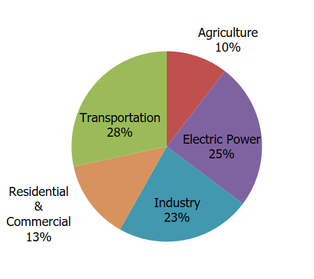
Total emissions in 2022 are 6,343.2 Million Metric Tons of CO₂ equivalent . Percentages may not add up to 100% due to independent rounding. Greenhouse gas emissions from the commercial, residential, and industrial sectors increase substantially when indirect emissions from electricity end-use are included, due to the relatively large share of electricity use by buildings (e.g., heating, ventilation, and air conditioning; lighting; appliances and plug load) and use of electricity for powering industrial machinery. More information is also in the electricity end-use emissions section of this page.

Land Use, Land-Use Change, and Forestry in the United States is a net sink and offsets 13% of these greenhouse gas emissions. This net sink is not shown in the above diagrams. All emission estimates are sourced from the Inventory of U.S. Greenhouse Gas Emissions and Sinks: 1990–2022 .

What are the primary sources of U.S. greenhouse gas emissions and sinks in each economic sector? :

• Transportation – Greenhouse gas emissions from transportation primarily come from burning fossil fuel for cars, trucks, ships, trains, and planes. Over 94% of the fuel used for transportation is petroleum based, which includes primarily gasoline and diesel and results in direct emissions. 2 The transportation sector is the largest source of direct greenhouse gas emissions and second largest source when indirect emissions from electricity end-use are allocated across sectors. The transportation sector is an end-use sector for electricity but currently represents a relatively low percentage of total electricity use. Indirect emissions from electricity are less than 1 percent of direct emissions.
• Electricity production – Electric power includes emissions from electricity production used by other end use sectors (e.g., industry). In 2022, 60% of our electricity comes from burning fossil fuels, mostly coal and natural gas. 3
• Industry – Greenhouse gas emissions from industry primarily come from burning fossil fuels for energy, as well as greenhouse gas emissions from certain chemical reactions necessary to produce goods from raw materials. Industrial emissions are the third largest source of direct emissions. If indirect emissions from electricity use are allocated to the industrial end-use sector (e.g. to power industrial buildings and equipment), industrial activities account for a much larger share of U.S. greenhouse gas emissions as shown above.
• Commercial and Residential – Greenhouse gas emissions from the commercial and residential sector come from fossil fuels burned for heat and the use of gases for refrigeration and cooling in buildings, and non-building specific emissions such as the handling of waste. The commercial and residential sector emissions increase substantially when indirect emissions from electricity end-use are included, largely because buildings use 75% of the electricity generated in the US (e.g., for heating, ventilation and air conditioning; lighting; appliances, and plug loads). 4 When emissions from electricity use are distributed to the commercial and residential end-use sector , commercial and residential activities account for a much larger share of U.S. greenhouse gas emissions as shown above.
• Agriculture – Greenhouse gas emissions from agriculture come from livestock such as cows, agricultural soils, and rice production. Indirect emissions from electricity use in agricultural activities (e.g., powering buildings and equipment) are about 5 percent of direct emissions.
• Land Use and Forestry – While not shown in the figure, land areas can act as a sink (absorbing CO 2 from the atmosphere) or a source of greenhouse gas emissions. In the United States, since 1990, managed forests and other lands are a net sink, i.e., they have absorbed more CO 2 from the atmosphere than they emit, offsetting 13% of total gross greenhouse gas emissions.

Since 1990, gross U.S. greenhouse gas emissions have decreased by just over 3%. From year to year, emissions can rise and fall due to changes in the economy, the price of fuel, and other factors. In 2022, U.S. greenhouse gas emissions increased 0.2% compared to 2021 levels. In 2020, there was a sharp decline in emissions largely due to the impacts of the coronavirus (COVID-19) pandemic on travel and other economic activity. In 2021 and 2022, the increase in total greenhouse gas emissions was driven largely by an increase in CO 2  emissions from fossil fuel combustion due to the continued rebound in economic activity after the height of the COVID-19 pandemic. In 2022, CO 2  emissions from fossil fuel combustion increased by 8% relative to 2020 and 1% relative to 2021. CO 2  emissions from natural gas consumption increased by 5% relative to 2021. CO 2  emissions from coal consumption decreased by 6% from 2021. The increase in natural gas consumption and emissions in 2022 is observed across all sectors except for U.S. Territories, while the coal decrease in primarily in the electric power sector. Emissions from petroleum use increased by less than 1% in 2022.

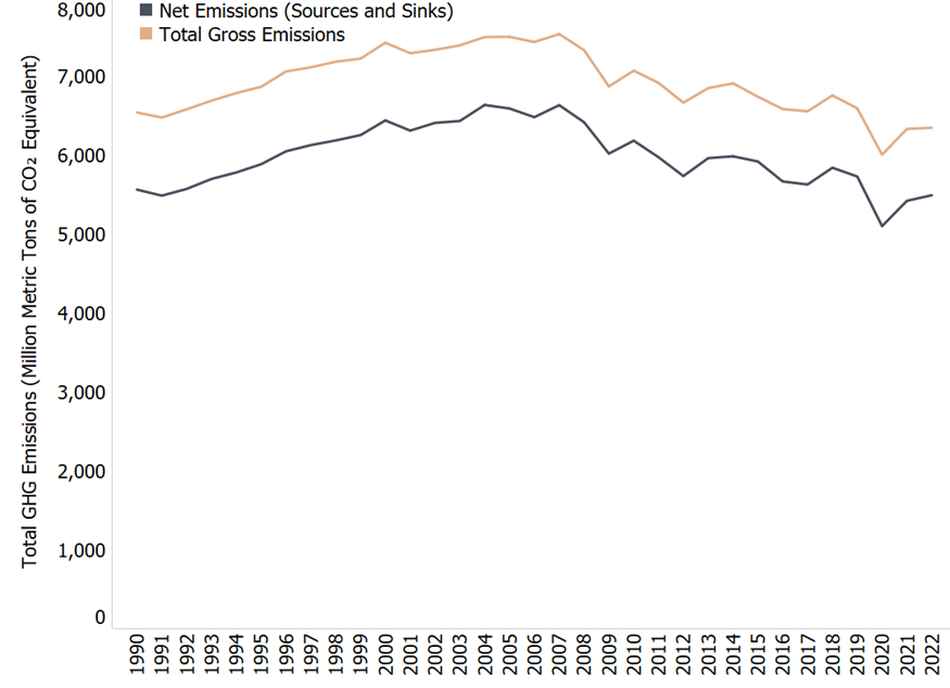
• IPCC (2013) Climate Change 2013: The Physical Science Basis . Contribution of Working Group I to the Fifth Assessment Report of the Intergovernmental Panel on Climate Change. [Stocker, T.F., D. Qin, G.K. Plattner, M. Tignor, S.K. Allen, J. Boschung, A. Nauels, Y. Xia, V. Bex and P.M. Midgley (eds.)]. Cambridge University Press, Cambridge, United Kingdom and New York, NY, USA, 1535 pp. .
• IPCC (2022): Climate Change 2022: Mitigation of Climate Change. Contribution of Working Group III to the Sixth Assessment Report of the Intergovernmental Panel on Climate Change [P.R. Shukla, J. Skea, R. Slade, A. Al Khourdajie, R. van Diemen, D. McCollum, M. Pathak, S. Some, P. Vyas, R. Fradera, M. Belkacemi, A. Hasija, G. Lisboa, S. Luz, J. Malley, (eds.)]. Cambridge University Press, Cambridge, UK and New York, NY, USA. doi: 10.1017/9781009157926
• U.S. Energy Information Administration (2023) .  Electricity Explained – Basics
• National Renewable Energy Laboratory (2023). NREL Researchers Reveal How Buildings Across United States Do—and Could—Use Energy. Shoemaker, Susannah.

Electric Power Sector Emissions

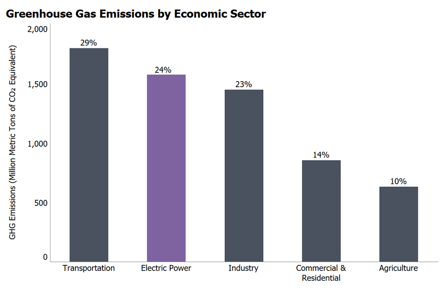
The Electricity power sector involves the generation, transmission, and distribution of electricity.  Carbon dioxide (CO 2 )  makes up the vast majority of greenhouse gas emissions from the sector, but smaller amounts of  methane (CH 4 )  and  nitrous oxide (N 2 O)  are also emitted. These gases are released during the combustion of fossil fuels, such as coal, oil, and natural gas, to produce electricity. Less than 1% of greenhouse gas emissions from the sector come from  sulfur hexafluoride (SF 6 ) , an insulating chemical used in electricity transmission and distribution equipment.

Greenhouse Gas Emissions in the Electric Power Sector by Fuel Source

Coal combustion is more carbon-intensive than burning natural gas or petroleum for electric power production. Although coal use accounted for 55% of CO 2  emissions from the sector, it represented only 20% of the electricity generated in the United States in 2022. Natural gas use accounted for 39% of electricity generation in 2022, and petroleum use accounted for less than 1%. The remaining generation in 2022 came from non-fossil fuel sources, including nuclear (19%) and renewable energy sources (21%), which include hydroelectricity, biomass, wind, and solar. 1  Most of these non-fossil sources, such as nuclear, hydroelectric, wind, and solar, are non-emitting.

Electric Power Sector Trends

In 2022, the electric power sector was the second largest source of U.S. greenhouse gas emissions, accounting for 25% of the U.S. total. Electric power sector emissions increased 7% in 2021. Greenhouse gas emissions from electric power production have decreased by about 15% since 1990 due to a shift in generation to lower- and non-emitting sources of electricity generation and an increase in end-use energy efficiency.

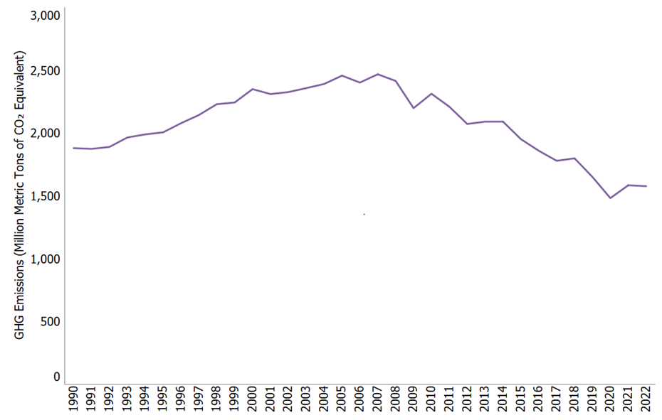
Greenhouse Gas Emissions by Electricity End-Use

Electricity is used by other end-use sectors—in homes, businesses, and factories—and the greenhouse gas emissions from electricity generation can be allocated to the sectors that use the electricity. Looking at greenhouse gas emissions by end-use sector can help us understand energy demand across sectors and changes in energy use over time.

When emissions from electric power generation are allocated to the industrial end-use sector, industrial activities account for a much larger share of U.S. greenhouse gas emissions. Greenhouse gas emissions from commercial and residential buildings also increase substantially when emissions from electricity end-use are included, due to the relatively large share of electricity use mostly building related (e.g., heating, ventilation, and air conditioning; lighting; and appliances) in these sectors. The transportation sector currently has a relatively low percentage of electricity use and thus indirect emissions, but it is growing due to the use of electric and plug-in vehicles.

Reducing Emissions from Electric Power Production

There are a variety of opportunities to reduce greenhouse gas emissions associated with electric power production, transmission, and distribution. The table below categorizes these opportunities and provides examples. For a more comprehensive list, see Chapter 6 (PDF) (88 pp, 3.6MB) of the Contribution of Working Group III to the Sixth Assessment Report of the Intergovernmental Panel on Climate Change . 2

• U.S. Energy Information Administration (2022). Electricity Explained - Basics.
• IPCC, 2022: Climate Change 2022: Mitigation of Climate Change. Contribution of Working Group III to the Sixth Assessment Report of the Intergovernmental Panel on Climate Change [P.R. Shukla, J. Skea, R. Slade, A. Al Khourdajie, R. van Diemen, D. McCollum, M. Pathak, S. Some, P. Vyas, R. Fradera, M. Belkacemi, A. Hasija, G. Lisboa, S. Luz, J. Malley, (eds.)]. Cambridge University Press, Cambridge, UK and New York, NY, USA. doi: 10.1017/9781009157926

Transportation Sector Emissions

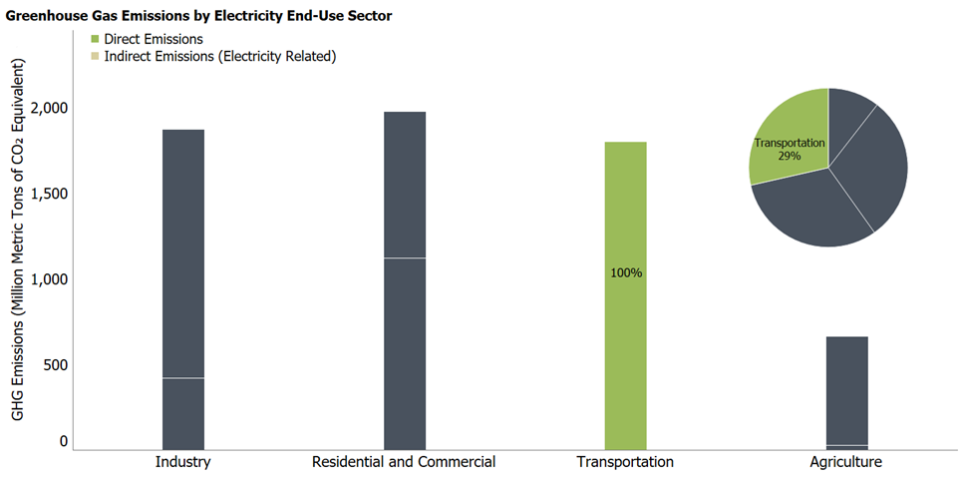
The Transportation sector includes the movement of people and goods by cars, trucks, trains, ships, airplanes, and other vehicles. The majority of greenhouse gas emissions from transportation are  carbon dioxide (CO 2 )  emissions resulting from the combustion of petroleum-based products, like gasoline and diesel fuel, in internal combustion engines. The largest sources of transportation-related greenhouse gas emissions include passenger cars, medium- and heavy-duty trucks, and light-duty trucks, including sport utility vehicles, pickup trucks, and minivans. These sources account for over half of the emissions from the transportation sector. The remaining greenhouse gas emissions from the transportation sector come from other modes of transportation, including commercial aircraft, ships, boats, and trains, as well as pipelines and lubricants. Indirect emissions from electricity are less than 1 percent of direct emissions. 

Relatively small amounts of methane (CH 4 ) and nitrous oxide (N 2 O) are emitted during fuel combustion. In addition, hydrofluorocarbon (HFC) emissions also occur from the Transportation sector. These emissions result from the use of mobile air conditioners and refrigerated transport.

Transportation Sector Emissions Trends

• Carbon Pollution from Transportation
• EPA and U.S. DOE Fuel Economy
• Smart Growth
• Renewable Fuel Standard
• U.S. Inventory's section on Fossil Fuel Combustion

In 2022, direct and indirect greenhouse gas emissions from transportation accounted for 29% of total U.S. greenhouse gas emissions, making it the third largest contributor of U.S. greenhouse gas emissions when considering indirect emissions from distributed electricity. When considering only direct emissions, transportation is the largest contributor of U.S. greenhouse gas emissions (28%). From 1990 to 2022, total transportation emissions from fossil fuel combustion increased by 19%. From 2021 to 2022, emissions decreased by less than 1%. The largest sources of transportation greenhouse gas emissions in 2022 were light-duty trucks, which include sport utility vehicles, pickup trucks, and minivans (37%); medium- and heavy-duty trucks (23%); passenger cars (20%); commercial aircraft (7%); other aircraft (2%); pipelines (4%); ships and boats (3%); and rail (2%). In terms of the overall trend, from 1990 to 2022, total transportation emissions have increased due, in large part, to increased demand for travel. The number of vehicle miles traveled (VMT) by light-duty motor vehicles (passenger cars and light-duty trucks) increased by 47% from 1990 to 2022, as a result of a confluence of factors including population growth, economic growth, urban sprawl, and periods of low fuel prices. Between 1990 and 2004, average fuel economy among new vehicles sold annually declined, as sales of light-duty trucks increased. Starting in 2005, average new vehicle fuel economy began to increase, while light-duty VMT grew only modestly for much of the period. Average new vehicle fuel economy has improved almost every year since 2005, slowing the rate of increase of CO 2  emissions.

Learn more about Greenhouse Gas Emissions from Transportation .

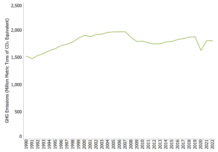
Reducing Emissions from Transportation

There are a variety of opportunities to reduce greenhouse gas emissions associated with transportation. The table shown below categorizes these opportunities and provides examples. For a more comprehensive list, see Chapter 10 of the Contribution of Working Group III to the Sixth Assessment Report of the Intergovernmental Panel on Climate Change . 1

Industry Sector Emissions

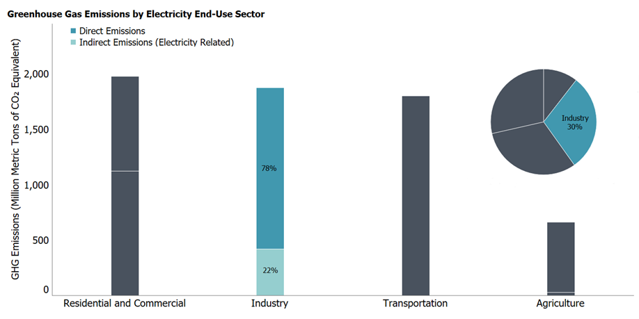
The Industry sector produces the goods and raw materials we use every day. The greenhouse gases emitted during industrial production are split into two categories: direct emissions that are produced at the facility, and indirect emissions that occur off site but are associated with the facility's use of electricity.

Direct emissions are produced by burning fuel for power or heat, through chemical reactions, and from leaks from industrial processes or equipment. Most direct emissions come from the consumption of fossil fuels for energy. A smaller amount of direct emissions, roughly one third, come from leaks from natural gas and petroleum systems, the use of fuels in production (e.g., petroleum products used to make plastics), and chemical reactions during the production of chemicals, metals (e.g., iron and steel), and minerals (e.g., cement).

Indirect emissions are produced by burning fossil fuel at a power plant to make electricity, which is then used by an industrial facility to power industrial buildings and machinery.

More information about facility-level emissions from large industrial sources is available through EPA's Greenhouse Gas Reporting Program data publication tool . National-level information about emissions from industry as a whole can be found in the sections on Fossil Fuel Combustion and the Industrial Processes chapter in the Inventory of U.S. Greenhouse Gas Emissions and Sinks .

Industry Sector Emissions Trends

In 2022, direct and indirect industrial greenhouse gas emissions accounted for 30% of total U.S. greenhouse gas emissions, making it the second largest contributor of greenhouse gas emissions of any sector. Direct greenhouse gas emissions from Industry account for 23% of total U.S. greenhouse gas emissions, making it the third largest contributor to direct U.S. greenhouse gas emissions, after the  Transportation  and  Electric Power  sectors. From 2021 to 2022, total energy use in the industrial sector decreased by less than 1%.Total U.S. greenhouse gas emissions from industry, including electricity, have declined by 22% since 1990.

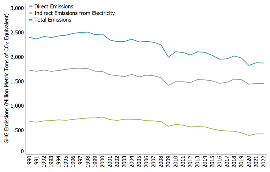
Reducing Emissions from Industry

There are a wide variety of industrial activities that cause greenhouse gas emissions, and many opportunities to reduce them. The table shown below provides some examples of opportunities for industry to reduce emissions. For a more comprehensive list, see Chapter 11 of the Contribution of Working Group III to the Sixth Assessment Report of the Intergovernmental Panel on Climate Change . 1

Commercial and Residential Sector Emissions

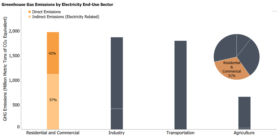
The Residential and Commercial sectors include all homes and commercial businesses (excluding agricultural and industrial activities). Greenhouse gas emissions from this sector come from  direct emissions  including fossil fuel combustion for heating and cooking needs, management of waste and wastewater, and leaks from refrigerants in homes and businesses, as well as  indirect emissions   from the use of electricity by homes and businesses (e.g., heating, ventilation, and air conditioning; lighting; and appliances, and plug loads). The building sector uses 75% of the electricity generated in the US1.

Direct emissions are produced from residential and commercial activities in a variety of ways:

• Combustion of natural gas and petroleum products for heating and cooking emits carbon dioxide (CO 2 ) , methane (CH 4 ) , and nitrous oxide (N 2 O) . Emissions from natural gas consumption represent 78% of the direct fossil fuel CO 2  emissions from the residential and commercial sector in 2022. Coal consumption is a minor component of energy use in both of these sectors.
• Organic waste sent to landfills emits CH 4 .
• Wastewater treatment plants emit CH 4 and N 2 O.
• Anaerobic digestion at biogas facilities emits CH 4 .
• Fluorinated gases (mainly hydrofluorocarbons, or HFCs) used in air conditioning and refrigeration systems can be released during servicing or from leaking equipment.

Indirect emissions are produced by burning fossil fuel at a power plant to make electricity, which is then used in residential and commercial activities, such as lighting and for appliances.

Note: Residential and commercial sector emissions presented here do not necessarily represent the full suite of emissions related to buildings and the broader built environment. The commercial and residential sectors numbers don’t include any emissions/sinks from production of construction materials (e.g., upstream emissions from production of cement, emissions and sinks from land use changes, etc.). Those would be reflected in other sectors. Also, as shown above, emissions from these sectors include other emissions that do not occur at the building site (i.e., landfills, etc.). Furthermore, energy use in these sectors may also include energy used for equipment (such as motor gasoline used for non-highway vehicles or lawn and garden equipment), exterior lighting, or construction. In addition, energy use for some large buildings, such as energy-intensive office buildings and factories with large onsite combustion, are typically included in industrial sector energy use.

More national-level information about emissions from the residential and commercial sector can be found in the U.S. Inventory's Trends in Greenhouse Gas Emissions and Energy chapters (Chapters 2 and 4 respectively).

Commercial and Residential Sector Emissions Trends

In 2022, direct and indirect greenhouse gas emissions from homes and businesses accounted for 31% of total U.S. greenhouse gas emissions. Direct emissions were 13% of total U.S. greenhouse gas emissions in 2022. Greenhouse gas emissions from homes and businesses vary from year to year, often correlated with annual fluctuations in energy use caused primarily by weather conditions. Total residential and commercial greenhouse gas emissions, including direct and indirect emissions, in 2022 have increased by less than 1% since 1990. Greenhouse gas emissions from on-site direct emissions in homes and businesses have increased by 8% since 1990. Additionally, indirect emissions from electricity use by homes and businesses increased from 1990 to 2007, but have decreased since then to approximately 4% below 1990 levels in 2021.

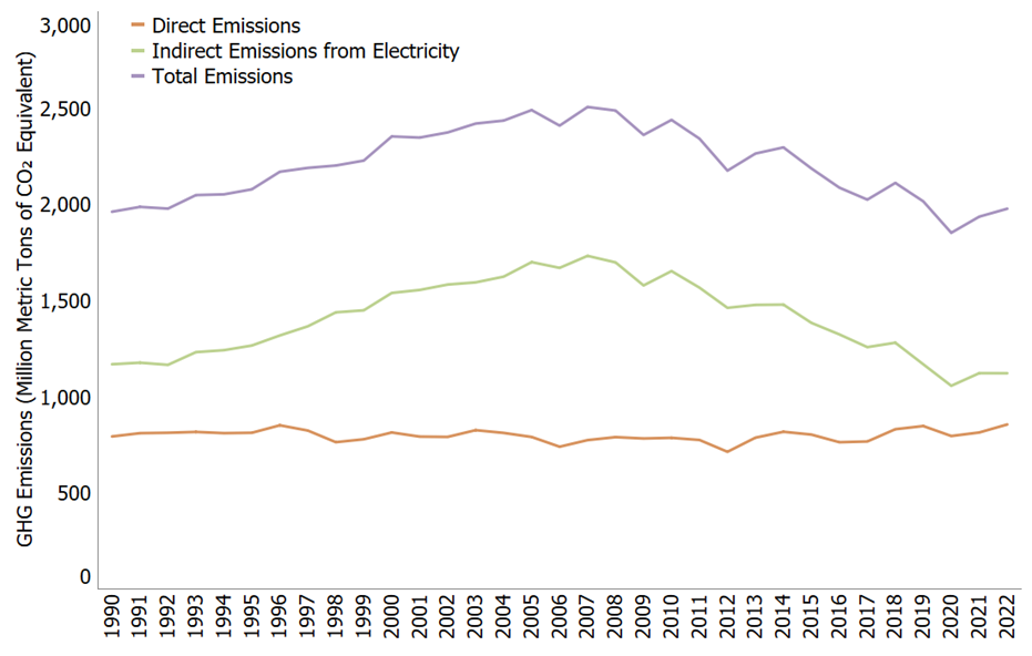
• National Renewable Energy Laboratory (2023). NREL Researchers Reveal How Buildings Across United States Do—and Could—Use Energy. Shoemaker, Susannah

Reducing Emissions from Homes and Businesses

The table shown below provides examples of opportunities to reduce emissions from homes and businesses. For a more comprehensive list of options and a detailed assessment of how each option affects different gases, see Chapter 9 and Chapter 12 of the Contribution of Working Group III to the Sixth Assessment Report of the Intergovernmental Panel on Climate Change .

Agriculture Sector Emissions

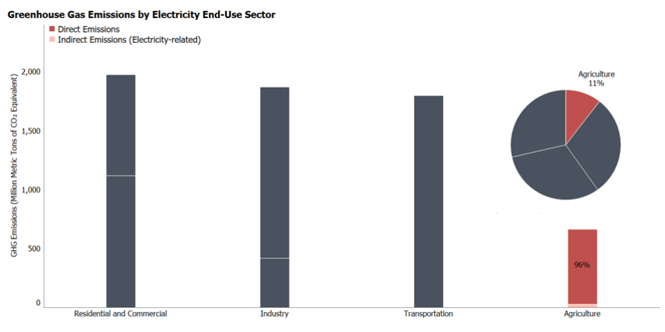
• Various management practices on agricultural soils can lead to increased availability of nitrogen in the soil and result in emissions of nitrous oxide (N 2 O) . Specific activities that contribute to N 2 O emissions from agricultural lands include the application of synthetic and organic fertilizers, the growth of nitrogen-fixing crops, the drainage of organic soils, and irrigation practices. Management of agricultural soils accounts for just over half of the greenhouse gas emissions from the Agriculture sector. Management of croplands and grasslands can also lead to emissions or sequestration of carbon dioxide (CO 2 ) . These emissions and removals are included under the Land Use, Land-Use Change, and Forestry sector .
• Livestock, especially ruminants such as cattle, produce methane (CH 4 ) as part of their normal digestive processes. This process is called enteric fermentation, and it represents over a quarter of the greenhouse gas emissions from the Agriculture sector.
• The way in which manure from livestock is managed also contributes to CH 4  and N 2 O emissions. Different manure treatment and storage methods affect how much of these greenhouse gases are produced. Manure management accounts for about 14% of the total greenhouse gas emissions from the Agriculture sector in the United States.
• Smaller sources of agricultural emissions include CO 2 from liming and urea application, CH 4 from rice cultivation, and burning crop residues, which produces CH 4 and N 2 O.

More information about emissions from agriculture can be found in the agriculture chapter in the Inventory of U.S. Greenhouse Gas Emissions and Sinks .

Agriculture Sector Emissions Trends

In 2022, direct greenhouse gas emissions from the agriculture sector accounted for 9.4% of total U.S. greenhouse gas emissions. Greenhouse gas emissions from agriculture have increased by 8% since 1990. Agricultural soil management activities, such as application of synthetic and organic fertilizers, deposition of livestock manure, and growing nitrogen fixing plants, were the largest contributors to U.S. N 2 O emissions in 2022, accounting for 75% of total N 2 O emissions. Emissions from other agricultural sources have generally remained flat or changed by a relatively small amount since 1990.

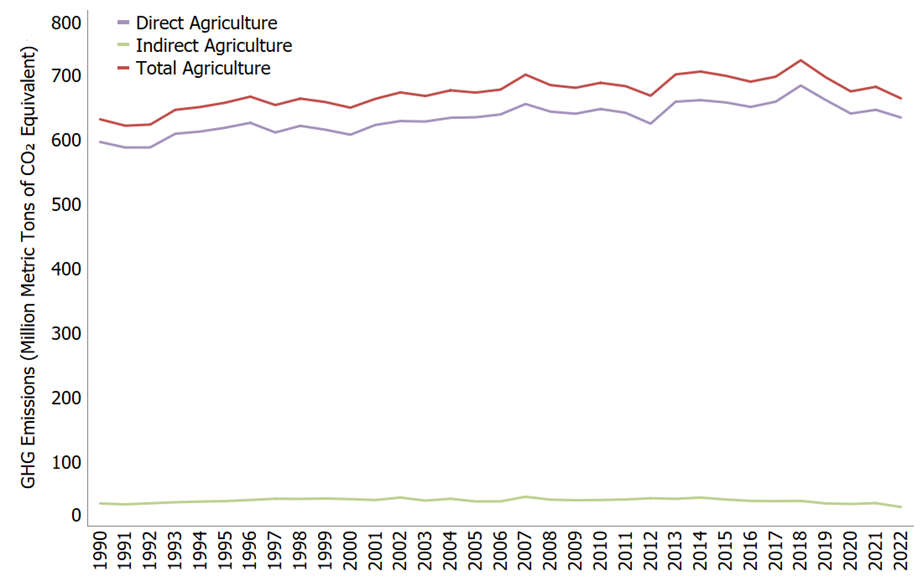
Reducing Emissions from Agriculture

The table shown below provides examples of opportunities to reduce emissions from agriculture. For a more comprehensive list of options and a detailed assessment of how each option affects different gases, see Chapter 7 of the Contribution of Working Group III to the Sixth Assessment Report of the Intergovernmental Panel on Climate Change .

Land Use, Land-Use Change, and Forestry Sector Emissions and Sequestration

Plants absorb carbon dioxide (CO 2 ) from the atmosphere as they grow, and they store some of this carbon as perennial aboveground and belowground biomass throughout their lifetime. Soils and dead organic matter/litter can also store some of the carbon from these plants depending on how the soil is managed and other environmental conditions (e.g., climate). This storage of carbon in plants, dead organic matter/litter and soils is called biological carbon sequestration. Because biological sequestration takes CO 2 out of the atmosphere and stores it in these carbon pools, it is also called a carbon "sink."

Emissions or sequestration of CO 2 , as well as emissions of CH 4 and N 2 O, can occur from management of lands in their current use or as lands are converted to other land uses. Carbon dioxide is exchanged between the atmosphere and the plants and soils on land, for example, as cropland is converted into grassland, as lands are cultivated for crops, or as forests grow. In addition, using biological feedstocks (such as energy crops or wood) for purposes such as electricity generation, as inputs to processes that create liquid fuels, or as building materials can lead to emissions or sequestration.*

In the United States overall, Land Use, Land-Use Change, and Forestry (LULUCF) activities have resulted in more removal of CO 2 from the atmosphere than emissions. Because of this, the LULUCF sector in the United States is considered a net sink, rather than a source, of CO 2 . In many areas of the world, the opposite is true, particularly in countries where large areas of forest land are cleared, often for conversion to agricultural purposes or for settlements. In these situations, the LULUCF sector can be a net source of greenhouse gas emissions.

• More national-level information about land use, land-use change, and forestry is available from the Land Use, Land-Use Change, and Forestry chapter in the Inventory of U.S. Greenhouse Gas Emissions and Sinks . For more information on emissions and sequestration from forest land and urban trees in settlement areas, see also the USDA's USFS Resource Bulletin .
• For more information about global emissions from land use and forestry activities, see EPA's Global Greenhouse Gas emissions page and the Contribution of Working Group III to the Fifth Assessment Report of the Intergovernmental Panel on Climate Change .

* Emissions and sequestration of CO 2 are presented under the Land Use, Land-Use Change, and Forestry sector in the Inventory. Emissions of methane (CH 4 ) and nitrous oxide (N 2 O) also occur as a result of land use and management activities in the LULUCF sector. Other emissions from CH 4 , and N 2 O are also presented in the Energy sector.

Emissions and Trends

In 2022, the net CO 2  removed from the atmosphere from the LULUCF sector was 13% of total U.S. greenhouse gas emissions. Between 1990 and 2022, total carbon sequestration in the LULUCF sector decreased by 11%, primarily due to a decrease in the rate of net carbon accumulation in forests, as well as an increase in CO 2  emissions from urbanization. Additionally, while episodic in nature, increased CO 2 , CH 4  and N 2 O emissions from forest fires have also occurred over the time series.

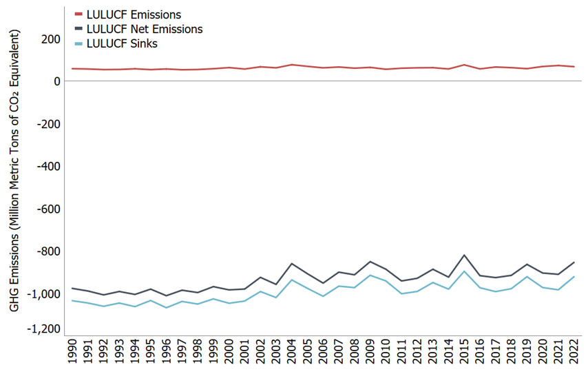
Reducing Emissions and Enhancing Sinks from Land Use, Land-Use Change, and Forestry

In the LULUCF sector, opportunities exist to reduce greenhouse gas emissions and increase the potential to sequester carbon from the atmosphere by enhancing sinks. The table shown below provides some examples of opportunities for both reducing emissions and enhancing sinks. For a more comprehensive list, see Chapter 7 of the Contribution of Working Group III to the Sixth Assessment Report of the Intergovernmental Panel on Climate Change .

6,343 million metric tons of CO 2 : What does that mean?

An explanation of units.

A million metric tons equals about 2.2 billion pounds, or 1 trillion grams. For comparison, a small car is likely to weigh a little more than 1 metric ton. Thus, a million metric tons are roughly the same mass as 1 million small cars!

The U.S. Inventory uses metric units for consistency and comparability with other countries. For reference, a metric ton is slightly more (approximately 10%) than a U.S. "short" ton.

Greenhouse gas emissions are often measured in carbon dioxide ( CO 2 ) equivalent . To convert emissions of a gas into CO 2 equivalent, its emissions are multiplied by the gas's Global Warming Potential (GWP) . The GWP takes into account the fact that many gases are more effective at warming Earth than CO 2 , per unit mass.

The GWP values appearing in the Overview of Greenhouse Gases and Sources of Greenhouse Gas web pages reflect the values used in the U.S. Inventory, which are drawn from the IPCC's Fifth Assessment Report (AR5). For further discussion of GWPs and an estimate of greenhouse gas emissions using updated GWPs, see Annex 6 of the U.S. Inventory and the IPCC's discussion on GWPs (PDF) (106 pp, 7.7MB).

• GHG Emissions and Removals Home
• Overview of Greenhouse Gases
• Sources of GHG Emissions and Removals
• Global Emissions and Removals
• National Emissions and Removals
• State and Tribal GHG Data and Resources
• Facility-Level Emissions
• Gridded Methane Emissions
• Carbon Footprint Calculator
• GHG Equivalencies Calculator
• Capacity Building for GHG Inventories

• Bioenergy Technologies Office
• Accomplishments
• National Biotechnology & Biomanufacturing Initiative
• Bold Goals for U.S. Biotechnology & Biomanufacturing
• 2023 Multi-Year Program Plan
• Bioproduct Production
• CO2 Utilization
• Deconstruction & Fractionation
• Synthesis & Upgrading
• Conversion Technologies Related Links
• Sustainability
• Data, Modeling, & Analysis Related Links
• Feedstock-Conversion Interface R&D
• Feedstock Technologies Related Links
• Algal Logistics
• Algal Production
• Algal Related Links
• Development
• Infrastructure
• Systems Development & Integration Related Links
• Sustainable Aviation Fuels
• Sustainable Marine Fuels
• Waste-to-Energy
• CO2 Reduction & Upgrading for e-Fuels Consortium
• Consortium for Computational Physics & Chemistry
• Co-Optimization of Fuels & Engines
• Feedstock-Conversion Interface Consortium
• Bioenergy FAQs
• Biofuel Basics
• Biopower Basics
• Bioproduct Basics
• Biomass Feedstocks
• Career Exploration Wheel
• Career Grid
• Workforce Training Opportunities Map
• Algae Technology Educational Consortium
• Workforce Development Strategy
• Bioenergy Jobs at BETO
• BRIDGES Events
• BRIDGES Webinar Recordings and Presentations
• Internships & Fellowships
• Teacher & Classroom Resources
• BioenergizeME Infographic Challenge
• Wood Heater Design Challenge
• Funding Opportunities
• Analytical Tools
• Bioenergy Publications
• Bioenergy Related Links
• State Biomass Contacts
• BioProse: Bioenergy R&D Blog
• Bioenergy News
• Bioeconomy 2020
• Bioeconomy 2018
• Bioeconomy 2017
• Bioenergy 2016
• Bioenergy 2015
• Biomass 2014
• Biomass 2013
• Biomass 2012
• Biomass 2011
• Inaccessible
• Biomass 2009
• Peer Review 2023
• Peer Review 2021
• Peer Review 2019
• Peer Review 2017
• Peer Review 2015
• Peer Review 2013
• Peer Review 2011
• Past Meetings & Workshops
• Bioenergy Newsletter

Earth Day is an opportunity to recognize the importance of nurturing and protecting our environment as we strive towards a greener, more equitable future for our planet. At the U.S. Department of Energy (DOE)  Bioenergy Technologies Office (BETO), contributions to a clean energy future are being made every day through research, development, and demonstration of technologies that mobilize domestic renewable carbon resources for the reduction of greenhouse gas (GHG) emissions across the U.S. economy.

BETO Technology Manager for  Renewable Carbon Resources (RCR), Dr. Chenlin Li, is a DOE innovator supercharging the clean energy revolution with a commitment to stewardship of the planet’s natural resources. BETO’s RCR Program focuses on facilitating availability, reducing cost, improving quality, and maximizing environmental benefits while mobilizing renewable carbon resources to enable the production of bioenergy and bioproducts. 

Dr. Li is a chemical and environmental engineer by training and demonstrates expertise at BETO by leading various renewable carbon feedstock supply chain, feedstock production, preprocessing, waste utilization technologies and collaborates with national laboratories, academic, government, and industry members to meet sustainability goals. On Earth Day, the work of Dr. Li can inspire us all to do our part to help create a better future.

Dr. Li’s Career Path

Dr. Li graduated from the University of Hong Kong in 2007 with a Ph.D. in environmental engineering. Her research focused on anaerobic fermentation of wastewater and solid wastes for bio-hydrogen and ethanol production. She received her Master’s (2002) and Bachelor’s (1999) degrees in chemical engineering from Zhengzhou University, China.

Dr. Li has had the opportunity to work for multiple DOE national laboratories during her career. “All together, over 13 years at three DOE national labs before joining BETO as a federal employee in August 2020, it has been an amazing and rewarding journey for me,” said Dr. Li. Prior to BETO, she joined  Idaho National Laboratory (INL) in January 2015 as a staff scientist in the Biofuels and Renewable Energy Technologies Department. Before joining INL, she worked at  Lawrence Berkeley National Laboratory from 2011 to 2015 as a research scientist and biomass deconstruction lead at the Advanced Biofuels/Bioproducts Process Demonstration Unit. She completed her postdoctoral research at  Sandia National Laboratories  and  Joint BioEnergy Institute (2008-2011) and Washington State University (2007-2008) on lignocellulosic biomass characterization and pretreatment technologies.

A Step into the Energy Transition: Partnering with INL for first-of-its-kind Biomass Feedstock Facility 

A major project under Dr. Li’s portfolio is her leadership role in launching INL’s upgraded  Biomass Feedstock National User Facility (BFNUF), a center for rapid technology development, testing and scaling up advanced biomass pre-processing toward the commercialization of biofuels and bioproducts.   DOE Secretary Jennifer Granholm participated in a ribbon-cutting ceremony in May 2023 for the $15 million expansion and upgrade that began in 2020 and was funded by BETO. The BFNUF will be a critical component of the  Clean Fuels & Products Shot™ efforts to decarbonize the transportation and chemical industries and is essential to achieving the Biden-Harris administration’s goals to reach net zero emissions economy-wide by 2050.

Before leading the project at BETO, Dr. Li did program management at INL and oversaw INL’s bioenergy R&D portfolio including BFNUF upgrading capabilities. “I was able to continue managing the project from the BETO side one year after I left INL and joined BETO, so I feel proud of the upgrade. This past May, the BFNUF opened the doors to welcome industry collaborators, academia, and federal agencies, with new biomass characterization and preprocessing capabilities, while also announcing the Clean Fuels and Products Earthshot™. INL did an awesome job from the scientists and engineers of the bioenergy program to the overall lab leadership team. The ribbon-cutting event turned out to be a great event and I was proud. Going through the process from the ideas and schematic design of the upgrading capabilities on paper to seeing the equipment and system operating efficiently in the upgraded facility was amazing,” said Dr. Li.

The facility helps the bioenergy industry overcome challenges related to turning renewable carbon resources like purpose-grown energy crops, municipal solid waste, forestry and agricultural residues into valuable fuels and clean chemicals.

BETO Portfolio and Environmental, Equity Impacts 

Dr. Li’s portfolio is extensive and focuses on climate smart agriculture with several on-going projects under her leadership with national laboratories and universities that are making an impact on the environment, equity, and workforce development. Her projects also support the recently released  2023 Billion-Ton Report , which shows that the U.S. could sustainably triple its production of biomass to more than 1 billion tons per year.

One of the collaborations in her portfolio is with  Pacific Northwest National Laboratory (PNNL) in partnership with Washington State University (WSU). This partnership is helping farmers with agricultural practices using cover crops. A cover crop is a plant that is used primarily to benefit the successful growth of other future crops, including help with soil health, soil erosion, increasing biodiversity, and other benefits to a farm. 

“The cover crop project at PNNL is very unique in terms of working with farmers to utilize cover crops as feedstocks for biofuels to maximize the value. Cover crops are grown in three weather systems/locations, wetland, dryland, and irrigated land, in Washington State in at least two growing seasons to understand the seasonal variability and impact of weather systems for optimal growth. PNNL and WSU are working directly with farmers to do field day education and generating relevant field data for cover crop adoption. They’re also providing information on economic and sustainability impacts to local and regional farmers,” said Dr. Li.

Dr. Li highlighted the benefits of this project to minority groups in Washington State with the research and collaboration bringing economic, education, and workforce opportunities to the local area. She shared that this project provides cover crop productivity data, harvesting strategies, cover crop properties for biofuel conversion, and cost and environmental sustainability benefits. “It also helps in gathering data on the utilization of cover crops such as blending with waste from different locations to supply sustainable feedstocks to biorefineries for biofuels production. There are many good things coming out of this project.”

Another project under Dr. Li’s portfolio involves researchers from  North Carolina State University , the  National Renewable Energy Laboratory (NREL), the  University of Puerto Rico , and the  Fearless Fund who want to turn wood waste from Hurricane Maria 6 years ago and excess seaweed on Caribbean shorelines into sustainable aviation fuel (SAF) and graphite, an important component in electric vehicle batteries. This  project has the potential to not only mitigate waste streams and harmful impact on coastal communities but create new jobs and stimulate underserved students’ interest in career pathways in the bioeconomy. 

In this project, there will be efforts to recruit graduate students from HBCUs, including North Carolina Agricultural & Technical College (A&T), NC Central University, and the  University of Puerto Rico . Training materials will be developed to assist students develop skills necessary to qualify for the jobs enabled by this project, and employment opportunities in the bioeconomy. The multi-institutional research team goal is to empower a region already impacted by climate change and often underrepresented in economic development.

Earth Day and Pursuing Renewable Energy Opportunities 

From cover crop projects to municipal solid waste, Dr. Li is passionate about the work she’s doing at BETO and Earth Day serves as a reminder that environmental sustainability is achievable. Dr. Li encourages individuals, including the next generation, to recognize environmental, energy, and equity justice opportunities as a career path. 

“I believe the most challenging part of career development is jumping out of your comfort zone and taking on challenges," said Dr. Li. "For those people that are very passionate about clean energy and climate change, I would say be willing to adapt to changes and have the courage to pursue paths that are very important.  Don’t limit yourself in trying different opportunities for career development.”

If you’re interested in learning more about career opportunities in bioenergy, visit BETO’s  Bioenergy Careers web page and  Internships and Fellowships web page. BETO's  Bioenergy Career Exploration Wheel is also available to explore bioenergy industry-related jobs.

NASA Mission Excels at Spotting Greenhouse Gas Emission Sources

Flaring, in which excess natural gas is intentionally burned into the air, is one way methane is released from oil and gas facilities. NASA’s EMIT mission, in more than a year in operation, has shown a proficiency at spotting emissions of methane and other greenhouse gases from space.

Since launching 16 months ago, the EMIT imaging spectrometer aboard the International Space Station has shown an ability to detect more than just surface minerals.

More than a year after first detecting methane plumes from its perch aboard the International Space Station, data from NASA’s EMIT instrument is now being used to identify point-source emissions of greenhouse gases with a proficiency that has surprised even its designers.

Short for Earth Surface Mineral Dust Source Investigation, EMIT was launched in July 2022 to map 10 key minerals on the surface of the world’s arid regions. Those mineral-related observations, which are already available to researchers and the public, will help improve understanding of how dust that gets lofted into the atmosphere affects climate.

Detecting methane was not part of EMIT’s primary mission, but the instrument’s designers did expect the imaging spectrometer to have the capability. Now, with more than 750 emissions sources identified since August 2022 – some small, others in remote locations, and others persistent in time – the instrument has more than delivered in that regard, according to a new study published in Science Advances .

“We were a little cautious at first about what we could do with the instrument,” said Andrew Thorpe, a research technologist on the EMIT science team at NASA’s Jet Propulsion Laboratory in Southern California and the paper’s lead author. “It has exceeded our expectations.”

EMIT identified a cluster of 12 methane plumes within a 150-square-mile (400-square-kilometer) area of southern Uzbekistan on Sept. 1, 2022. The instrument captured the cluster within a single shot, called a scene by researchers.

By knowing where methane emissions are coming from, operators of landfills, agriculture sites, oil and gas facilities, and other methane producers have an opportunity to address them. Tracking human-caused emissions of methane is key to limiting climate change because it offers a comparatively low-cost, rapid approach to reducing greenhouse gases. Methane lingers in the atmosphere for about a decade, but during this span, it’s up to 80 times more powerful at trapping heat than carbon dioxide, which remains for centuries.

Surprising Results

EMIT has proven effective at spotting emission sources both big (tens of thousands of pounds of methane per hour) and surprisingly small (down to the hundreds of pounds of methane per hour). This is important because it permits identification of a greater number of “super-emitters” – sources that produce disproportionate shares of total emissions.

The new study documents how EMIT, based on its first 30 days of greenhouse gas detection, can observe 60% to 85% of the methane plumes typically seen in airborne campaigns.

In a remote corner of southeastern Libya, EMIT on Sept. 3, 2022, detected a methane plume that was emitting about 979 pounds (444 kilograms) per hour. It’s one of the smallest sources detected so far by the instrument.

From several thousand feet above the ground, methane-detecting instruments on aircraft are more sensitive, but to warrant sending a plane, researchers need prior indication that they’ll detect methane. Many areas are not examined because they are considered too remote, too risky, or too costly. Additionally, the campaigns that do occur cover relatively limited areas for short periods.

On the other hand, from about 250 miles (400 kilometers) altitude on the space station, EMIT collects data over a large swath of the planet – specifically the arid regions that fall between 51.6 degrees north and south latitude. The imaging spectrometer captures 50-mile-by-50-mile (80-kilometer-by-80-kilometer) images of the surface – researchers call them “scenes” – including many regions that have been beyond the reach of airborne instruments.

This time-lapse video shows the Canadarm2 robotic arm of the International Space Station maneuvering NASA’s EMIT mission onto the exterior of the station. Extraction from the SpaceX Dragon spacecraft began around 5:15 p.m. PDT on July 22 and was completed at 10:15 a.m. PDT on July 24. Portions of the installation have been omitted, while others have been speeded up.

“The number and scale of methane plumes measured by EMIT around our planet is stunning,” said Robert O. Green, a JPL senior research scientist and EMIT’s principal investigator.

Scene-by-Scene Detections

To support source identification, the EMIT science team creates maps of methane plumes and releases them on a website , with underlying data available at the joint NASA-United States Geological Survey Land Processes Distributed Active Archive Center ( LP DAAC ). The mission’s data is available for use by the public, scientists, and organizations.

Since EMIT began collecting observations in August 2022, it has documented over 50,000 scenes. The instrument spotted a cluster of emissions sources in a rarely studied region of southern Uzbekistan on Sept. 1, 2022, detecting 12 methane plumes totaling about 49,734 pounds (22,559 kilograms) per hour.

In addition, the instrument has spotted plumes far smaller than expected. Captured in a remote corner of southeastern Libya on Sept. 3, 2022, one of the smallest sources so far was emitting 979 pounds (444 kilograms) per hour, based on estimates of local wind speed.

More About the Mission

EMIT was selected from the Earth Venture Instrument-4 solicitation under the Earth Science Division of NASA’s Science Mission Directorate and was developed at NASA’s Jet Propulsion Laboratory, which is managed for the agency by Caltech in Pasadena, California. The instrument’s data is available at the NASA Land Processes Distributed Active Archive Center for use by other researchers and the public.

To learn more about the mission, visit:

https://earth.jpl.nasa.gov/emit/

News Media Contact

Andrew Wang / Jane J. Lee

Jet Propulsion Laboratory, Pasadena, Calif.

626-379-6874 / 818-354-0307

[email protected] / [email protected]

Monroe County agriculture: This is the wettest April in six years

Weather for the second half of April may be warmer with more rain forecast, according to the National Weather Service Climate Prediction Center. Its eight- to 14-day outlook for April 24-30, updated April 16, is calling for a 65 percent chance of above normal temperatures and a 25 percent chance of above normal precipitation. Rainfall at the MSU Enviroweather site in Deerfield had recorded 3.19 inches of rain as of April 16, with more rain forecast. This is by far the wettest month of April of the past six years at this location. Minimum soil temperatures were in the low 50s on April 15-16, suitable for planting unless the rain is cold, which will greatly slow down germination.  Growing degree day (heat units) are the second highest of the past six years through the first half of April.  

Earth Day was Monday, although a celebration will be held at Monroe County Community College on Saturday, April 27. First recognized in 1970, Earth Day serves as a reminder of everyone’s responsibility to safeguard the environment, the land, water, soil and air. Some easy things that everyone can do include: reducing the use of single-use containers, particularly plastic; recycle many items through the Monroe County Health Department; and re-use items. The 2024 Healthy Monroe Recycling events calendar was recently mailed to all residential customers and includes medication take back, electronics recycling, weekly single-stream recycling, household hazardous waste collection, secure document shredding and tire recycling collections. For questions about any of this, contact Dan Rock at 734-240-7909.  

Agricultural greenhouse gas emissions fell to their lowest levels in 10 years, according to an Environmental Protection Agency April 11 published report of the inventory of U.S. Greenhouse Gas Emissions and Sinks: 1990-2022. U.S. agriculture represents just under 10 percent of total U.S. emissions when compared to other sectors of the economy, with livestock-related emissions bout three percent. 

Additional MDARD pesticide exams will be offered April 30 in Owosso and May 15 in Hillsdale. Interested people can register through MSU Event Management at: events.anr.msu.edu/2024RUPInPersonTesting/ . A review session will be held in the morning from 8:30 a.m. to 12:30 p.m. at a cost of $15. Then, participants will be able to take: the Private Core exam, the Commercial Core exam, the Fumigation Standard exam or the Aerial Standard exam.   All commercial category exams must be taken through the Metro Institute and MDARD. MCCC is one site to take these computer-based exams.

Subscribe Now: For all the latest local developments, breaking news and high school sports content.

Arbor Day is Friday, April 26, and, much like Earth Day, celebrates nature. Started by Julius Sterling Morton, the first Arbor Day occurred on April 10, 1872, in Nebraska City, Neb. A popular Arbor Day tradition is to plant a tree in honor or memory of someone. Trees help clean our air and water, provide shade and have a calming effect. Trees support wildlife and an entire ecosystem, including birds, animals and provide people with powerful medicine, materials for living and agriculture. Trees are a big ally in climate, pulling carbon dioxide from the air, putting the carbon in the soil and releasing oxygen. Trees can have great value to property owners. I have read that one tree, in a Washington, D.C., neighborhood, increased the value of the property by $100,000.

Thank you for visiting nature.com. You are using a browser version with limited support for CSS. To obtain the best experience, we recommend you use a more up to date browser (or turn off compatibility mode in Internet Explorer). In the meantime, to ensure continued support, we are displaying the site without styles and JavaScript.

• View all journals
• Explore content
• About the journal
• Publish with us
• Sign up for alerts
• Published: 31 October 2012

One-third of our greenhouse gas emissions come from agriculture

• Natasha Gilbert  

Nature ( 2012 ) Cite this article

21k Accesses

71 Citations

1162 Altmetric

Metrics details

• Climate change
• Climate sciences
• Developing world
• Plant sciences

Farmers advised to abandon vulnerable crops in face of climate change.

The global food system, from fertilizer manufacture to food storage and packaging, is responsible for up to one-third of all human-caused greenhouse-gas emissions, according to the latest figures from the Consultative Group on International Agricultural Research (CGIAR), a partnership of 15 research centres around the world.

In two reports published today 1 , 2 , the CGIAR says that reducing agriculture’s carbon footprint is central to limiting climate change. And to help to ensure food security, farmers across the globe will probably have to switch to cultivating more climate-hardy crops and farming practices.

“The food-related emissions and the impacts of climate change on agriculture and the food system will profoundly alter the way we grow and produce food,” says Sonja Vermeulen, a plant scientist at the University of Copenhagen in Denmark and a co-author of one of the studies, which estimates the emissions footprint of food 1 . 

Vermeulen and her colleagues examined for the first time the carbon emissions for all stages of the global food system. Previous work has only looked at the contribution of agricultural production to greenhouse-gas emissions, including the release of nitrous oxide from soils from farming techniques such as tilling.

Using estimates from 2005, 2007 and 2008, the researchers found that agricultural production provides the lion’s share of greenhouse-gas emissions from the food system, releasing up to 12,000 megatonnes of carbon dioxide equivalent a year — up to 86% of all food-related anthropogenic greenhouse-gas emissions. Next is fertilizer manufacture, which releases up to 575 megatonnes, followed by refrigeration, which emits 490 megatonnes. The researchers found that the whole food system released 9,800–16,900 megatonnes of carbon dioxide equivalent into the atmosphere in 2008, including indirect emissions from deforestation and land-use changes.

“This is the first time this has been done. It’s a brave paper, considering the huge data limitations — this is why there is such a big range,” said Bruce Campbell, an ecologist and director of the CGIAR research programme on climate change, agriculture and food security.

In high-income countries such as the United Kingdom, post-production — including storage and transport — contributes a large proportion of the food system’s greenhouse-gas emissions, whereas in China, for example, fertilizer manufacture has the biggest role, the researchers found.

Increasing temperatures and the likelihood of flooding will challenge farmers’ ability to safely store and distribute food, boosting the risk of food-borne illnesses and diarrhoeal diseases, they add.

“Food safety will in future be a crucial issue. This is a different take from the usual focus on crop yields and emissions,” says Campbell.

In the second report 2 , Philip Thornton, an agricultural scientist at the International Livestock Research Institute,headquartered in Nairobi, Kenya, examined the potential effects of climate change on 22 of the world’s most important agricultural commodities, including wheat, soya beans and potatoes.

By 2050, climate change could cause irrigated wheat yields in developing countries to drop by 13%, and irrigated rice could fall by 15%. In Africa, maize yields could drop by 10–20% over the same time frame.

For some crops, improvements to heat resistance through conventional and transgenic breeding, for example, will help farmers to adapt. But for others, more radical changes are needed. Thornton says that potato-growing areas, including China and India, are likely to see yields drop significantly as temperatures rise, and he suggests that farmers consider growing crops, such as bananas, that do better in warmer climates.

Campbell says that the CGIAR will use the paper to help set its research agenda for the next decade and “identify which crops and which regions to focus investment on”.

He calls on governments meeting next month at the climate-change conference in Doha, Qatar, to agree on a way forward to tackle the challenges of mitigating and adapting to the effects of climate change on agriculture.

Vermeulen, S. J., Campbell, B. M. & Ingram, J. S. I. Annu. Rev. Environ. Resour. 37 , 195–222 (2012).

Article   Google Scholar  

Thornton, P. Recalibrating Food Production in the Developing World: Global Warming Will Change More Than Just the Climate. CCAFS Policy Brief no. 6. (CGIAR Research Program on Climate Change, Agriculture and Food Security, 2012).

Download references

You can also search for this author in PubMed   Google Scholar

Related links

Related links in nature research.

Summit urged to clean up farming 2011-Nov-16

Climate-smart agriculture is needed 2011-Mar-02

Intensive farming may ease climate change 2010-Jun-15

Related external links

Climate Chnage conference, Doha

Rights and permissions

Reprints and permissions

About this article

Cite this article.

Gilbert, N. One-third of our greenhouse gas emissions come from agriculture. Nature (2012). https://doi.org/10.1038/nature.2012.11708

Download citation

Published : 31 October 2012

DOI : https://doi.org/10.1038/nature.2012.11708

Share this article

Anyone you share the following link with will be able to read this content:

Sorry, a shareable link is not currently available for this article.

Provided by the Springer Nature SharedIt content-sharing initiative

This article is cited by

Dynamic modeling and techno-economic assessment of hybrid renewable energy and thermal storage systems for a net-zero energy greenhouse in south korea.

• Misbaudeen Aderemi Adesanya
• Abdulfatai Olatunji Yakub
• Hyun-Woo Lee

Clean Technologies and Environmental Policy (2024)

Enhancing the bioconversion rate and end products of black soldier fly (BSF) treatment – A comprehensive review

• Shahida Anusha Siddiqui
• Ito Fernando

Environment, Development and Sustainability (2024)

Use of Mulches in Various Tillage Conditions Reduces the Greenhouse Gas Emission—an Overview

• Syed Tanveer Shah
• Abdul Basit
• Ayesha Sohrab

Gesunde Pflanzen (2023)

The nexuses between carbon emissions, agriculture production efficiency, research and development, and government effectiveness: evidence from major agriculture-producing countries

• Rizwana Yasmeen
• Caihong Tang

Environmental Science and Pollution Research (2022)

Soil carbon stock in olive groves agroforestry systems under different management and soil characteristics

• Camilla Bateni
• Maurizio Ventura
• Andrea Pisanelli

Agroforestry Systems (2021)

Quick links

• Explore articles by subject
• Guide to authors
• Editorial policies

Sign up for the Nature Briefing: Anthropocene newsletter — what matters in anthropocene research, free to your inbox weekly.