what visual presentation goes with an ordinal data

We use essential cookies to make Venngage work. By clicking “Accept All Cookies”, you agree to the storing of cookies on your device to enhance site navigation, analyze site usage, and assist in our marketing efforts.

Manage Cookies

Cookies and similar technologies collect certain information about how you’re using our website. Some of them are essential, and without them you wouldn’t be able to use Venngage. But others are optional, and you get to choose whether we use them or not.

Strictly Necessary Cookies

These cookies are always on, as they’re essential for making Venngage work, and making it safe. Without these cookies, services you’ve asked for can’t be provided.

Show cookie providers

• Google Login

Functionality Cookies

These cookies help us provide enhanced functionality and personalisation, and remember your settings. They may be set by us or by third party providers.

Performance Cookies

These cookies help us analyze how many people are using Venngage, where they come from and how they're using it. If you opt out of these cookies, we can’t get feedback to make Venngage better for you and all our users.

• Google Analytics

Targeting Cookies

These cookies are set by our advertising partners to track your activity and show you relevant Venngage ads on other sites as you browse the internet.

• Google Tag Manager
• Infographics
• Daily Infographics
• Graphic Design
• Graphs and Charts
• Data Visualization
• Human Resources
• Training and Development
• Beginner Guides

Blog Graphic Design

15 Effective Visual Presentation Tips To Wow Your Audience

By Krystle Wong , Sep 28, 2023

So, you’re gearing up for that big presentation and you want it to be more than just another snooze-fest with slides. You want it to be engaging, memorable and downright impressive. 

Well, you’ve come to the right place — I’ve got some slick tips on how to create a visual presentation that’ll take your presentation game up a notch. 

Packed with presentation templates that are easily customizable, keep reading this blog post to learn the secret sauce behind crafting presentations that captivate, inform and remain etched in the memory of your audience.

Click to jump ahead:

What is a visual presentation & why is it important?

15 effective tips to make your visual presentations more engaging, 6 major types of visual presentation you should know , what are some common mistakes to avoid in visual presentations, visual presentation faqs, 5 steps to create a visual presentation with venngage.

A visual presentation is a communication method that utilizes visual elements such as images, graphics, charts, slides and other visual aids to convey information, ideas or messages to an audience. 

Visual presentations aim to enhance comprehension engagement and the overall impact of the message through the strategic use of visuals. People remember what they see, making your point last longer in their heads. 

Without further ado, let’s jump right into some great visual presentation examples that would do a great job in keeping your audience interested and getting your point across.

In today’s fast-paced world, where information is constantly bombarding our senses, creating engaging visual presentations has never been more crucial. To help you design a presentation that’ll leave a lasting impression, I’ve compiled these examples of visual presentations that will elevate your game.

1. Use the rule of thirds for layout

Ever heard of the rule of thirds? It’s a presentation layout trick that can instantly up your slide game. Imagine dividing your slide into a 3×3 grid and then placing your text and visuals at the intersection points or along the lines. This simple tweak creates a balanced and seriously pleasing layout that’ll draw everyone’s eyes.

2. Get creative with visual metaphors

Got a complex idea to explain? Skip the jargon and use visual metaphors. Throw in images that symbolize your point – for example, using a road map to show your journey towards a goal or using metaphors to represent answer choices or progress indicators in an interactive quiz or poll.

3. Visualize your data with charts and graphs

The right data visualization tools not only make content more appealing but also aid comprehension and retention. Choosing the right visual presentation for your data is all about finding a good match. 

For ordinal data, where things have a clear order, consider using ordered bar charts or dot plots. When it comes to nominal data, where categories are on an equal footing, stick with the classics like bar charts, pie charts or simple frequency tables. And for interval-ratio data, where there’s a meaningful order, go for histograms, line graphs, scatterplots or box plots to help your data shine.

In an increasingly visual world, effective visual communication is a valuable skill for conveying messages. Here’s a guide on how to use visual communication to engage your audience while avoiding information overload.

4. Employ the power of contrast

Want your important stuff to pop? That’s where contrast comes in. Mix things up with contrasting colors, fonts or shapes. It’s like highlighting your key points with a neon marker – an instant attention grabber.

5. Tell a visual story

Structure your slides like a storybook and create a visual narrative by arranging your slides in a way that tells a story. Each slide should flow into the next, creating a visual narrative that keeps your audience hooked till the very end.

Icons and images are essential for adding visual appeal and clarity to your presentation. Venngage provides a vast library of icons and images, allowing you to choose visuals that resonate with your audience and complement your message. 

6. Show the “before and after” magic

Want to drive home the impact of your message or solution? Whip out the “before and after” technique. Show the current state (before) and the desired state (after) in a visual way. It’s like showing a makeover transformation, but for your ideas.

7. Add fun with visual quizzes and polls

To break the monotony and see if your audience is still with you, throw in some quick quizzes or polls. It’s like a mini-game break in your presentation — your audience gets involved and it makes your presentation way more dynamic and memorable.

8. End with a powerful visual punch

Your presentation closing should be a showstopper. Think a stunning clip art that wraps up your message with a visual bow, a killer quote that lingers in minds or a call to action that gets hearts racing.

9. Engage with storytelling through data

Use storytelling magic to bring your data to life. Don’t just throw numbers at your audience—explain what they mean, why they matter and add a bit of human touch. Turn those stats into relatable tales and watch your audience’s eyes light up with understanding.

10. Use visuals wisely

Your visuals are the secret sauce of a great presentation. Cherry-pick high-quality images, graphics, charts and videos that not only look good but also align with your message’s vibe. Each visual should have a purpose – they’re not just there for decoration. 

11. Utilize visual hierarchy

Employ design principles like contrast, alignment and proximity to make your key info stand out. Play around with fonts, colors and placement to make sure your audience can’t miss the important stuff.

12. Engage with multimedia

Static slides are so last year. Give your presentation some sizzle by tossing in multimedia elements. Think short video clips, animations, or a touch of sound when it makes sense, including an animated logo . But remember, these are sidekicks, not the main act, so use them smartly.

13. Interact with your audience

Turn your presentation into a two-way street. Start your presentation by encouraging your audience to join in with thought-provoking questions, quick polls or using interactive tools. Get them chatting and watch your presentation come alive.

When it comes to delivering a group presentation, it’s important to have everyone on the team on the same page. Venngage’s real-time collaboration tools enable you and your team to work together seamlessly, regardless of geographical locations. Collaborators can provide input, make edits and offer suggestions in real time. 

14. Incorporate stories and examples

Weave in relatable stories, personal anecdotes or real-life examples to illustrate your points. It’s like adding a dash of spice to your content – it becomes more memorable and relatable.

15. Nail that delivery

Don’t just stand there and recite facts like a robot — be a confident and engaging presenter. Lock eyes with your audience, mix up your tone and pace and use some gestures to drive your points home. Practice and brush up your presentation skills until you’ve got it down pat for a persuasive presentation that flows like a pro.

Venngage offers a wide selection of professionally designed presentation templates, each tailored for different purposes and styles. By choosing a template that aligns with your content and goals, you can create a visually cohesive and polished presentation that captivates your audience.

Looking for more presentation ideas ? Why not try using a presentation software that will take your presentations to the next level with a combination of user-friendly interfaces, stunning visuals, collaboration features and innovative functionalities that will take your presentations to the next level. 

Visual presentations come in various formats, each uniquely suited to convey information and engage audiences effectively. Here are six major types of visual presentations that you should be familiar with:

1. Slideshows or PowerPoint presentations

Slideshows are one of the most common forms of visual presentations. They typically consist of a series of slides containing text, images, charts, graphs and other visual elements. Slideshows are used for various purposes, including business presentations, educational lectures and conference talks.

2. Infographics

Infographics are visual representations of information, data or knowledge. They combine text, images and graphics to convey complex concepts or data in a concise and visually appealing manner. Infographics are often used in marketing, reporting and educational materials.

Don’t worry, they are also super easy to create thanks to Venngage’s fully customizable infographics templates that are professionally designed to bring your information to life. Be sure to try it out for your next visual presentation!

3. Video presentation

Videos are your dynamic storytellers. Whether it’s pre-recorded or happening in real-time, videos are the showstoppers. You can have interviews, demos, animations or even your own mini-documentary. Video presentations are highly engaging and can be shared in both in-person and virtual presentations .

4. Charts and graphs

Charts and graphs are visual representations of data that make it easier to understand and analyze numerical information. Common types include bar charts, line graphs, pie charts and scatterplots. They are commonly used in scientific research, business reports and academic presentations.

Effective data visualizations are crucial for simplifying complex information and Venngage has got you covered. Venngage’s tools enable you to create engaging charts, graphs,and infographics that enhance audience understanding and retention, leaving a lasting impression in your presentation.

5. Interactive presentations

Interactive presentations involve audience participation and engagement. These can include interactive polls, quizzes, games and multimedia elements that allow the audience to actively participate in the presentation. Interactive presentations are often used in workshops, training sessions and webinars.

Venngage’s interactive presentation tools enable you to create immersive experiences that leave a lasting impact and enhance audience retention. By incorporating features like clickable elements, quizzes and embedded multimedia, you can captivate your audience’s attention and encourage active participation.

6. Poster presentations

Poster presentations are the stars of the academic and research scene. They consist of a large poster that includes text, images and graphics to communicate research findings or project details and are usually used at conferences and exhibitions. For more poster ideas, browse through Venngage’s gallery of poster templates to inspire your next presentation.

Different visual presentations aside, different presentation methods also serve a unique purpose, tailored to specific objectives and audiences. Find out which type of presentation works best for the message you are sending across to better capture attention, maintain interest and leave a lasting impression. 

To make a good presentation , it’s crucial to be aware of common mistakes and how to avoid them. Without further ado, let’s explore some of these pitfalls along with valuable insights on how to sidestep them.

Overloading slides with text

Text heavy slides can be like trying to swallow a whole sandwich in one bite – overwhelming and unappetizing. Instead, opt for concise sentences and bullet points to keep your slides simple. Visuals can help convey your message in a more engaging way.

Using low-quality visuals

Grainy images and pixelated charts are the equivalent of a scratchy vinyl record at a DJ party. High-resolution visuals are your ticket to professionalism. Ensure that the images, charts and graphics you use are clear, relevant and sharp.

Choosing the right visuals for presentations is important. To find great visuals for your visual presentation, Browse Venngage’s extensive library of high-quality stock photos. These images can help you convey your message effectively, evoke emotions and create a visually pleasing narrative. 

Ignoring design consistency

Imagine a book with every chapter in a different font and color – it’s a visual mess. Consistency in fonts, colors and formatting throughout your presentation is key to a polished and professional look.

Reading directly from slides

Reading your slides word-for-word is like inviting your audience to a one-person audiobook session. Slides should complement your speech, not replace it. Use them as visual aids, offering key points and visuals to support your narrative.

Lack of visual hierarchy

Neglecting visual hierarchy is like trying to find Waldo in a crowd of clones. Use size, color and positioning to emphasize what’s most important. Guide your audience’s attention to key points so they don’t miss the forest for the trees.

Ignoring accessibility

Accessibility isn’t an option these days; it’s a must. Forgetting alt text for images, color contrast and closed captions for videos can exclude individuals with disabilities from understanding your presentation. 

Relying too heavily on animation

While animations can add pizzazz and draw attention, overdoing it can overshadow your message. Use animations sparingly and with purpose to enhance, not detract from your content.

Using jargon and complex language

Keep it simple. Use plain language and explain terms when needed. You want your message to resonate, not leave people scratching their heads.

Not testing interactive elements

Interactive elements can be the life of your whole presentation, but not testing them beforehand is like jumping into a pool without checking if there’s water. Ensure that all interactive features, from live polls to multimedia content, work seamlessly. A smooth experience keeps your audience engaged and avoids those awkward technical hiccups.

Presenting complex data and information in a clear and visually appealing way has never been easier with Venngage. Build professional-looking designs with our free visual chart slide templates for your next presentation.

What software or tools can I use to create visual presentations?

You can use various software and tools to create visual presentations, including Microsoft PowerPoint, Google Slides, Adobe Illustrator, Canva, Prezi and Venngage, among others.

What is the difference between a visual presentation and a written report?

The main difference between a visual presentation and a written report is the medium of communication. Visual presentations rely on visuals, such as slides, charts and images to convey information quickly, while written reports use text to provide detailed information in a linear format.

How do I effectively communicate data through visual presentations?

To effectively communicate data through visual presentations, simplify complex data into easily digestible charts and graphs, use clear labels and titles and ensure that your visuals support the key messages you want to convey.

Are there any accessibility considerations for visual presentations?

Accessibility considerations for visual presentations include providing alt text for images, ensuring good color contrast, using readable fonts and providing transcripts or captions for multimedia content to make the presentation inclusive.

Most design tools today make accessibility hard but Venngage’s Accessibility Design Tool comes with accessibility features baked in, including accessible-friendly and inclusive icons.

How do I choose the right visuals for my presentation?

Choose visuals that align with your content and message. Use charts for data, images for illustrating concepts, icons for emphasis and color to evoke emotions or convey themes.

What is the role of storytelling in visual presentations?

Storytelling plays a crucial role in visual presentations by providing a narrative structure that engages the audience, helps them relate to the content and makes the information more memorable.

How can I adapt my visual presentations for online or virtual audiences?

To adapt visual presentations for online or virtual audiences, focus on concise content, use engaging visuals, ensure clear audio, encourage audience interaction through chat or polls and rehearse for a smooth online delivery.

What is the role of data visualization in visual presentations?

Data visualization in visual presentations simplifies complex data by using charts, graphs and diagrams, making it easier for the audience to understand and interpret information.

How do I choose the right color scheme and fonts for my visual presentation?

Choose a color scheme that aligns with your content and brand and select fonts that are readable and appropriate for the message you want to convey.

How can I measure the effectiveness of my visual presentation?

Measure the effectiveness of your visual presentation by collecting feedback from the audience, tracking engagement metrics (e.g., click-through rates for online presentations) and evaluating whether the presentation achieved its intended objectives.

Ultimately, creating a memorable visual presentation isn’t just about throwing together pretty slides. It’s about mastering the art of making your message stick, captivating your audience and leaving a mark.

Lucky for you, Venngage simplifies the process of creating great presentations, empowering you to concentrate on delivering a compelling message. Follow the 5 simple steps below to make your entire presentation visually appealing and impactful:

1. Sign up and log In: Log in to your Venngage account or sign up for free and gain access to Venngage’s templates and design tools.

2. Choose a template: Browse through Venngage’s presentation template library and select one that best suits your presentation’s purpose and style. Venngage offers a variety of pre-designed templates for different types of visual presentations, including infographics, reports, posters and more.

3. Edit and customize your template: Replace the placeholder text, image and graphics with your own content and customize the colors, fonts and visual elements to align with your presentation’s theme or your organization’s branding.

4. Add visual elements: Venngage offers a wide range of visual elements, such as icons, illustrations, charts, graphs and images, that you can easily add to your presentation with the user-friendly drag-and-drop editor.

5. Save and export your presentation: Export your presentation in a format that suits your needs and then share it with your audience via email, social media or by embedding it on your website or blog .

So, as you gear up for your next presentation, whether it’s for business, education or pure creative expression, don’t forget to keep these visual presentation ideas in your back pocket.

Feel free to experiment and fine-tune your approach and let your passion and expertise shine through in your presentation. With practice, you’ll not only build presentations but also leave a lasting impact on your audience – one slide at a time.

Presenting Data in Graphic Form

Ashley Crossman

• Statistics Tutorials
• Probability & Games
• Descriptive Statistics
• Inferential Statistics
• Applications Of Statistics
• Math Tutorials
• Pre Algebra & Algebra
• Exponential Decay
• Worksheets By Grade

Many people find frequency tables, crosstabs, and other forms of numerical statistical results intimidating. The same information can usually be presented in graphical form, which makes it easier to understand and less intimidating. Graphs tell a story with visuals rather than in words or numbers and can help readers understand the substance of the findings rather than the technical details behind the numbers.

There are numerous graphing options when it comes to presenting data. Here we will take a look at the most popularly used: pie charts , bar graphs , statistical maps, histograms, and frequency polygons.

A pie chart is a graph that shows the differences in frequencies or percentages among categories of a nominal or ordinal variable. The categories are displayed as segments of a circle whose pieces add up to 100 percent of the total frequencies.

Pie charts are a great way to graphically show a frequency distribution. In a pie chart, the frequency or percentage is represented both visually and numerically, so it is typically quick for readers to understand the data and what the researcher is conveying.

Like a pie chart, a bar graph is also a way to visually show the differences in frequencies or percentages among categories of a nominal or ordinal variable. In a bar graph, however, the categories are displayed as rectangles of equal width with their height proportional to the frequency of percentage of the category.

Unlike pie charts, bar graphs are very useful for comparing categories of a variable among different groups. For example, we can compare marital status among U.S. adults by gender. This graph would, thus, have two bars for each category of marital status: one for males and one for females. The pie chart does not allow you to include more than one group. You would have to create two separate pie charts, one for females and one for males.

Statistical Maps

Statistical maps are a way to display the geographic distribution of data. For example, let’s say we are studying the geographic distribution of the elderly persons in the United States. A statistical map would be a great way to visually display our data. On our map, each category is represented by a different color or shade and the states are then shaded depending on their classification into the different categories.

In our example of the elderly in the United States, let’s say we had four categories, each with its own color: Less than 10 percent (red), 10 to 11.9 percent (yellow), 12 to 13.9 percent (blue), and 14 percent or more (green). If 12.2 percent of Arizona’s population is over 65 years old, Arizona would be shaded blue on our map. Likewise, if Florida’s has 15 percent of its population aged 65 and older, it would be shaded green on the map.

Maps can display geographical data on the level of cities, counties, city blocks, census tracts, countries, states, or other units. This choice depends on the researcher’s topic and the questions they are exploring.

A histogram is used to show the differences in frequencies or percentages among categories of an interval-ratio variable. The categories are displayed as bars, with the width of the bar proportional to the width of the category and the height proportional to the frequency or percentage of that category. The area that each bar occupies on a histogram tells us the proportion of the population that falls into a given interval. A histogram looks very similar to a bar chart, however, in a histogram, the bars are touching and may not be of equal width. In a bar chart, the space between the bars indicates that the categories are separate.

Whether a researcher creates a bar chart or a histogram depends on the type of data he or she is using. Typically, bar charts are created with qualitative data (nominal or ordinal variables) while histograms are created with quantitative data (interval-ratio variables).

Frequency Polygons

A frequency polygon is a graph showing the differences in frequencies or percentages among categories of an interval-ratio variable. Points representing the frequencies of each category are placed above the midpoint of the category and are joined by a straight line. A frequency polygon is similar to a histogram, however, instead of bars, a point is used to show the frequency and all the points are then connected with a line.

Distortions in Graphs

When a graph is distorted, it can quickly deceive the reader into thinking something other than what the data really says. There are several ways that graphs can be distorted.

Probably the most common way that graphs get distorted is when the distance along the vertical or horizontal axis is altered in relation to the other axis. Axes can be stretched or shrunk to create any desired result. For example, if you were to shrink the horizontal axis (X axis), it could make the slope of your line graph appear steeper than it actually is, giving the impression that the results are more dramatic than they are. Likewise, if you expanded the horizontal axis while keeping the vertical axis (Y axis) the same, the slope of the line graph would be more gradual, making the results appear less significant than they really are.

When creating and editing graphs, it is important to make sure the graphs do not get distorted. Oftentimes, it can happen by accident when editing the range of numbers in an axis, for example. Therefore it is important to pay attention to how the data comes across in the graphs and make sure the results are being presented accurately and appropriately, so as to not deceive the readers.

Resources and Further Reading

• Frankfort-Nachmias, Chava, and Anna Leon-Guerrero. Social Statistics for a Diverse Society . SAGE, 2018.
• What Is a Bar Graph?
• How Bar Graphs Are Used to Display Data
• What Is a Histogram?
• Relative Frequency Histograms
• Make a Histogram in 7 Simple Steps
• What Are Pie Charts and Why Are They Useful?
• Lesson Plan: Survey Data and Graphing
• 7 Graphs Commonly Used in Statistics
• What Is a Two-Way Table of Categorical Variables?
• Frequencies and Relative Frequencies
• How and When to Use a Circle or Pie Graph
• Histogram Classes
• How to Discuss Charts and Graphs in English
• What Are Time Series Graphs?
• Tallies and Counts in Statistics
• Maximum and Inflection Points of the Chi Square Distribution

Sociology 3112

Department of sociology, main navigation, graphic presentation, learning objectives.

• Create and interpret a frequency table
• Determine when relative frequencies, cumulative frequencies and cumulative percentages are helpful/appropriate and when they are not
• Create and interpret a pie chart, a bar chart and a histogram, and determine which types of data are most appropriate for each

Frequency: the number of times a given observation appears in the data Frequency distribution: a table reporting the number of observations falling into each category of the variable Cumulative frequency distribution: a distribution showing the number of observations falling at or below each category, interval or score of a given variable. It is essentially a running total of frequencies. Cumulative percent distribution: a distribution showing the percentage of observations falling at or below each category, interval or score of a given variable.

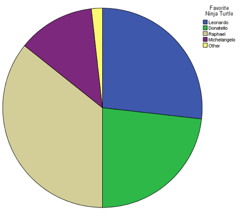
Last spring, I asked all the students in my class to name their favorite Teenage Mutant Ninja Turtle. The results were as follows:

Leonardo = 15 Donatello = 13 Raphael = 20 Michelangelo = 7 Other = 1 (One student put "Galapagos tortoise," either because he didn't understand the question or because he was being glib.)

The frequency (f) of a particular observation is the number of times the observation occurs in the data. In this example, the frequency of the Leonardo category is 15 because 15 people said he was their favorite. The distribution of a variable is the pattern of frequencies of the observation. A frequency distribution is a table that reports the number of observations that fall into each category of the variable we're analyzing. Making a frequency distribution for my Ninja Turtle data is pretty straightforward:

Favorite Ninja Turtle

Frequency distributions can show either the actual number of observations falling in each category or the percentage of observations. The actual number is called the raw score, while a distribution that includes the percentage of observations is called a relative frequency distribution. Relative frequency distributions are referred to as such because they allow for comparison between categories with unequal numbers of observations. We can turn the above table into a relative frequency distribution by calculating the percentage of observations in each category:

Relative frequencies can be useful when comparing the distributions of two different samples. Last fall, I asked my students the same question about their favorite Ninja Turtles, and the results are as follows:

Suppose we wanted to compare the popularity of Donatello between my two classes. We can see from looking at the raw frequencies that 13 of the students in my class last spring listed Donatello as their favorite, and 13 of the students in my class last fall did as well. Can we therefore conclude that Donatello was equally popular in both classes? No! We can't compare raw frequencies directly because the two groups have different sample sizes. My class last spring had 56 students, while my class last fall only had 40. In stats terminology, we would say that n=56 in the first sample, while n=40 in the second. In order to compare the two, we need to calculate the relative frequencies of the second sample:

Even though the same number of students in each class listed Donatello as their favorite Ninja Turtle, a higher percentage (i.e., a greater relative frequency) of students listed him as their favorite in the second sample.

Because "favorite Ninja Turtle" is a nominal variable, it would be just as easy to display these data as a pie chart. This pie chart shows the distribution of "favorite Ninja Turtle" among my class from last spring:

Pie charts are generally best for nominal-level variables, which are not ordered, while bar graphs are generally best for ordinal-level variables, which are ordered. This is because bar graphs allow us to display the categories in order from least to greatest. Consider the following made-up graph of the distribution of students in a fictional class by grade level:

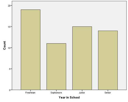
A bar chart allows us to display the frequency of each category while simultaneously keeping the categories in order from lowest to highest. Graphs and charts like these are usually used for nominal or ordinal variables that have relatively few categories. With interval/ratio level variables like GDP that typically have many more categories, there are better ways of summarizing information, which we will begin to talk about in the next chapter. I could make a pie chart illustrating the GDP for all 195 countries on the planet, but it would look pretty messy (it would have 195 slices).

Cumulative Frequencies

With interval/ratio variables, we can take our analysis a little further. The following table represents the annual income data taken from the fourth wave of the National Survey of Adolescent Health (the Add Health dataset).

Annual Income

This table is very similar to the above examples, but with one important difference. Both "Favorite Ninja Turtle" and "Year in School" have a relatively small number of categories, while income does not. I suppose I could display the information in terms of the nearest whole dollar, but that would probably give me one category for each of the 4,721 respondents, which would make for a comically large—and not terribly informative—table. To solve this problem, I collapsed the data into intervals. These intervals are often known as "class intervals," and are almost always used to summarize interval ratio data. In this case, we could say the width of the class interval is 5,000 (except for some of the larger intervals, which have a width of 10,000 or 24,000). There is no hard-and-fast rule for how wide to make the intervals; it usually falls to the discretion of whoever made the table.

With interval/ratio data, we can add two columns to the above table: cumulative frequency and cumulative percent. Cumulative frequency represents the number of observations that fall at or below a given interval, while cumulative percent represents the percent of observations that fall at or below a given interval. Please note: Including cumulative frequency and cumulative percent in a table only makes sense when dealing with variables that can be ranked from least to greatest. Including cumulative frequency and cumulative percent when describing a nominal-level variable is totally illogical. It's literally asking, "How many people are black or above?" or "How many people are Catholic or below?" Here's an example of a table with a cumulative frequency column:

To calculate the cumulative frequency for a given interval, we simply add the frequencies of that interval to all the intervals above it. For example, to calculate the cumulative frequency for the 5,000-9,000 interval, I added that interval's frequency (117) to that of all the intervals above it (134). In other words, 134+117 = 251. The same process holds true for any other interval. For the 25,000-29,000 interval, we simply add that interval's frequency (269) to those of all the intervals above it: 269+234+167+172+117+134 = 1,193. We can interpret that number by saying 1,093 of the people in our sample make $29,000 or less per year.

Calculating the cumulative percent follows essentially the same process except we sum the percentages rather than the number of observations. Consider the following table:

This table contains the same information as the previous tables, but the cumulative percent column allows for easier interpretation. For example, we could say that 23.16 percent of the people in our sample make $29,000 per year or less.

Rather than using bar graphs or pie charts, we can display interval/ratio data as a histogram. Some people (mistakenly) use the terms bar chart and histogram synonymously—they are not the same thing. The main difference between a histogram and a bar chart is this: in the case of the histogram, the distance between the bars (or bins, or buckets—there are a bunch of different names) is meaningful. In the bar graph used to illustrate grade level, for example, the distance between the categories isn't meaningful; in other words, you can't subtract a junior from a senior and get a freshman. In a histogram, however, the distance between intervals is meaningful. Consider the following histogram, which illustrates the distribution of ages from the New Immigrant Survey:

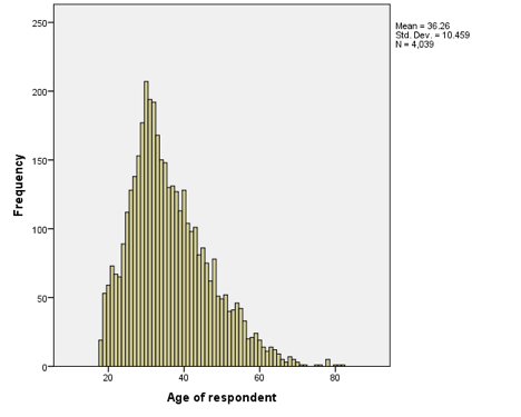
In this case, the distance between intervals is meaningful. Someone who is 60 years old is exactly 20 years older than someone who is 40. In other words, the further away the bars are from one another, the greater the difference between them.

Main Points

Frequency tables, pie charts, bar charts and histograms are all means of summarizing and displaying data. Determining the best or most appropriate way of displaying data depends largely on the level of measurement of the variable in question. Nominal-level variables can be displayed as frequency tables, but you should only include raw and relative frequencies (cumulative frequency and cumulative percent are inappropriate for use with nominal-level data). Nominal-level data can also be displayed as either pie charts or bar charts. Frequency tables displaying ordinal-level data can include raw frequencies, relative frequencies, cumulative frequencies and cumulative percentages. Like nominal-level data, ordinal-level data can be summarized with either pie charts or bar charts, though bar charts are arguably more effective. Frequency tables containing interval/ratio-level data can include all of the same components as those containing ordinal-level data, though they often include class intervals in order to make them easier to interpret. Interval/ratio-level data are the only data for which histograms are appropriate.

Tables, Charts and Graphs in SPSS

Before we start, there's one more thing about SPSS that I would like you to keep in mind. SPSS gives you a lot of options. SPSS gives you so many options, in fact, that even relatively simple procedures are needlessly complicated by superfluous buttons, drop-down menus and tabs. As you work through this section (and the manual in general), I would encourage you to ignore everything that isn't specifically included in the instructions.

Begin by downloading and opening the Add Health dataset. To create a frequency table, simply click on "Analyze," then "Descriptive Statistics," and then "Frequencies." Select the variable for which you would like to create a frequency table, and then move it into the (currently empty) "Variables" box by clicking on the arrow pointing to the right. Now click "Okay." The "Output" window should now pop up to display your frequency table. If you chose to make a frequency table for an interval/ratio variable, your table is probably several pages long, a fact that may lead you to (correctly) suspect that there must be better ways of summarizing interval/ratio data. We'll tackle that issue in the next chapter.

To create any sort of a graph (pie chart, bar graph or histogram), you'll need to click on "Graphs" and select "Legacy Dialogs" from the drop-down menu. You may be tempted to select "Chart Builder," but try to ignore it for now. The pop-out menu under "Legacy Dialogs" offers several different options in terms of graph creation, but we will focus on pie charts, bar charts and histograms.

First, let's make a pie chart. Under "Legacy Dialogs" select "Pie." A dialog box will open, giving you a choice between "Summaries for Groups of Cases," "Summaries of Separate Variables," and "Values of Individual Cases." Select the first option and click "Define." In the next dialog box, choose the variable you would like to see plotted in the pie chart, and move it into the space labeled "Define Slices by." Now click "Okay." A pie chart of the variable you chose should appear in your output window. If at any point you decide your chart doesn't quite look right, you can double click on the chart itself to open the chart editor. The chart editor allows you to change the colors of your charts, add backgrounds and add/remove labels. If you have a minute, I recommend playing around with it.

Now we'll make a bar graph. Under "Legacy Dialogs" select "Bar." Select "Simple" if you wish to have bars or lines of only one color displayed on the graph, in which case each bar or line will represent the relative frequency of the others. Choosing "Clustered" and "Stacked" will divide one variable into subgroups based on the level of a second variable (i.e., comparing different levels of educational attainment by race). Again, choose "Summaries for Groups of Cases" and click okay. Choose the variable you would like to see plotted on a bar graph and move it into the box labeled "Category Axis." If you chose to make either a clustered or stacked bar graph, you will also need to place a variable in the box labeled either "Display Clusters by" or "Display Stacks by." Once all the variables are in place, click "Okay" and a bar graph will appear in your output window.

Finally, let's make a histogram. Under "Legacy Dialogs" select "Histogram." Choose the variable you would like to see displayed in the histogram, and move it to the box labeled "Variable." Remember, histograms are only used with interval/ratio (a.k.a. "scale") variables, so choose your variable accordingly. Click "Okay," and a histogram should appear in your output window. Please enjoy this video walkthrough:

• Using the ADD Health dataset, create a pie chart for the "RACE" variable. Double click on your chart, and use the chart editor to change the colors of the slices and/or background.
• Create a frequency table for "GENDER." Approximately what percent of the respondents are female? Note that SPSS automatically displays a "Cumulative Percent" column. Does that make sense with a variable like "GENDER?" Hint: think of the level of measurement (nominal, ordinal or interval/ratio).
• Choose your favorite ordinal-level variable and make both a pie chart and a simple bar graph. Which do you think is easier to interpret? Are there any advantages to using one over the other?
• Create a clustered bar graph that shows "TVTIME" divided into groups by "RACE." In other words, create a clustered bar graph in which you place "TVTIME" in the "Category Axis" box and "RACE" in the "Display clusters by" box. Now interpret the graph. Do there appear to be any differences in the amount of time spent watching TV per day across racial groups?
• Finally, using the NIS dataset, create a histogram of the "AGE" variable. Which age(s) appear to have the highest frequency(ies)?

What Is Ordinal Data?

What is ordinal data, how is it used, and how do you collect and analyze it? Find out in this comprehensive guide.

Whether you’re new to data analytics or simply need a refresher on the fundamentals, a key place to start is with the four types of data. Also known as the four levels of measurement , this data analytics term describes the level of detail and precision with which data is measured. The four types (or scales) of data are:

• nominal data
• ordinal data
• interval data

In this article, I’m going to dive deep into ordinal data.

If the concept of these data types is completely new to you, we’ll start with a quick summary of the four different types, and then explore the various aspects of ordinal data in a bit more detail,

If you’d like to learn more data analytics skills, try our free 5-day data short course .

I’ll cover the following topics:

• An introduction to the four different types of data
• What is ordinal data? A definition

What are some examples of ordinal data?

• How is ordinal data collected and what is it used for?
• How to analyze ordinal data
• Summary and further reading

Ready to get your head around ordinal data? Then let’s get going!

1. An introduction to the four different types of data

To analyze a dataset, you first need to determine what type of data you’re dealing with.

Fortunately, to make this easier, all types of data fit into one of four broad categories: nominal , ordinal , interval, and ratio data. While these are commonly referred to as ‘data types,’ they are really different scales or levels of measurement .

Each level of measurement indicates how precisely a variable has been counted, determining the methods you can use to extract information from it. The four data types are not always clearly distinguishable; rather, they belong to a hierarchy. Each step in the hierarchy builds on the one before it.

The first two types of data, known as categorical data , are nominal and ordinal. These two scales take relatively imprecise measures.

While this makes them easier to analyze, it also means they offer less accurate insights. The next two types of data are interval and ratio. These are both types of numerical data , which makes them more complex. They are more difficult to analyze but have the potential to offer much richer insights.

• Nominal data is the simplest data type. It classifies data purely by labeling or naming values e.g. measuring marital status, hair, or eye color. It has no hierarchy to it.
• Ordinal data classifies data while introducing an order, or ranking. For instance, measuring economic status using the hierarchy: ‘wealthy’, ‘middle income’ or ‘poor.’ However, there is no clearly defined interval between these categories.
• Interval data classifies and ranks data but also introduces measured intervals. A great example is temperature scales, in Celsius or Fahrenheit. However, interval data has no true zero, i.e. a measurement of ‘zero’ can still represent a quantifiable measure (such as zero Celsius, which is simply another measure on a scale that includes negative values).
• Ratio data is the most complex level of measurement. Like interval data, it classifies and ranks data, and uses measured intervals. However, unlike interval data, ratio data also has a true zero. When a variable equals zero, there is none of this variable. A good example of ratio data is the measure of height—you cannot have a negative measure of height.

You’ll find a comprehensive guide to the four levels of data measurement here .

What do the different levels of measurement tell you?

Distinguishing between the different levels of measurement is sometimes a little tricky.

However, it’s important to learn how to distinguish them, because the type of data you’re working with determines the statistical techniques you can use to analyze it. Data analysis involves using descriptive analytics (to summarize the characteristics of a dataset) and inferential statistics (to infer meaning from those data).

These comprise a wide range of analytical techniques, so before collecting any data, you should decide which level of measurement is best for your intended purposes.

2. What is ordinal data? A definition

Ordinal data is a type of qualitative (non-numeric) data that groups variables into descriptive categories.

A distinguishing feature of ordinal data is that the categories it uses are ordered on some kind of hierarchical scale, e.g. high to low. On the levels of measurement, ordinal data comes second in complexity, directly after nominal data.

While ordinal data is more complex than nominal data (which has no inherent order) it is still relatively simplistic.

For instance, the terms ‘wealthy’, ‘middle income’, and ‘poor’ may give you a rough idea of someone’s economic status, but they are an imprecise measure–there is no clear interval between them. Nevertheless, ordinal data is excellent for ‘sticking a finger in the wind’ if you’re taking broad measures from a sample group and fine precision is not a requirement.

While ordinal data is non-numeric, it’s important to understand that it can still contain numerical figures. However, these figures can only be used as categorizing labels, i.e. they should have no inherent mathematical value.

For instance, if you were to measure people’s economic status you could use number 3 as shorthand for ‘wealthy’, number 2 for ‘middle income’, and number 1 for ‘poor.’ At a glance, this might imply numerical value, e.g. 3 = high and 1 = low. However, the numbers are only used to denote sequence. You could just as easily switch 3 with 1, or with ‘A’ and ‘B’ and it would not change the value of what you’re ordering; only the labels used to order it.

Key characteristics of ordinal data

• Ordinal data are categorical (non-numeric) but may use numbers as labels.
• Ordinal data are always placed into some kind of hierarchy or order (hence the name ‘ordinal’—a good tip for remembering what makes it unique!)
• While ordinal data are always ranked, the values do not have an even distribution .
• Using ordinal data, you can calculate the following summary statistics: frequency distribution, mode and median, and the range of variables.

What’s the difference between ordinal data and nominal data?

While nominal and ordinal data are both types of non-numeric measurement, nominal data have no order or sequence.

For instance, nominal data may measure the variable ‘marital status,’ with possible outcomes ‘single’, ‘married’, ‘cohabiting’, ‘divorced’ (and so on). However, none of these categories are ‘less’ or ‘more’ than any other. Another example might be eye color. Meanwhile, ordinal data always has an inherent order.

If a qualitative dataset lacks order, you know you’re dealing with nominal data.

3. What are some examples of ordinal data?

• Economic status (poor, middle income, wealthy)
• Income level in non-equally distributed ranges ($10K-$20K, $20K-$35K, $35K-$100K)
• Course grades (A+, A-, B+, B-, C)
• Education level (Elementary, High School, College, Graduate, Post-graduate)
• Likert scales (Very satisfied, satisfied, neutral, dissatisfied, very dissatisfied)
• Military ranks (Colonel, Brigadier General, Major General, Lieutenant General)
• Age (child, teenager, young adult, middle-aged, retiree)

As is hopefully clear by now, ordinal data is an imprecise but nevertheless useful way of measuring and ordering data based on its characteristics. Next up, let’s see how ordinal data is collected and how it generally tends to be used.

4. How is ordinal data collected and what is it used for?

Ordinal data are usually collected via surveys or questionnaires. Any type of question that ranks answers using an explicit or implicit scale can be used to collect ordinal data. An example might be:

• Question: Which best describes your knowledge of the Python programming language? Possible answers: Beginner, Basic, Intermediate, Advanced, Expert.

This commonly recognized type of ordinal question uses the Likert Scale, which we described briefly in the previous section. Another example might be:

• Question: To what extent do you agree that data analytics is the most important job for the 21st century? Possible answers: Strongly agree, Agree, Neutral, Disagree, Strongly Disagree.

It’s worth noting that the Likert Scale is sometimes used as a form of interval data. However, this is strictly incorrect. That’s because Likert Scales use discrete values , while interval data uses continuous values with a precise interval between them.

The distinctions between values on an ordinal scale, meanwhile, lack clear definition or separation, i.e. they are discrete. Although this means the values are imprecise and do not offer granular detail about a population, they are an excellent way to draw easy comparisons between different values in a sample group.

How is ordinal data used?

Ordinal data are commonly used for collecting demographic information.

This is particularly prevalent in sectors like finance, marketing, and insurance, but it is also used by governments, e.g. the census, and is generally common when conducting customer satisfaction surveys (in any industry).

5. How to analyze ordinal data

As discussed, the level of measurement you use determines the kinds of analysis you can carry out on your data. In general, these fall into two broad categories: descriptive statistics and inferential statistics.

We use descriptive statistics to summarize the characteristics of a dataset. This helps us spot patterns. Meanwhile, inferential statistics allow us to make predictions (or infer future trends) based on existing data. However, depending on the measurement scale, there are limits. You can learn more about the difference between descriptive and inferential statistics here .

For now, though, Let’s see what kinds of descriptive and inferential statistics you can measure using ordinal data.

Descriptive statistics for ordinal data

The descriptive statistics you can obtain using ordinal data are:

Frequency distribution

Measures of central tendency: mode and/or median, measures of variability: range.

Now let’s look at each of these in more depth.

Frequency distribution describes how your ordinal data are distributed.

For instance, let’s say you’ve surveyed students on what grade they’ve received in an examination. Possible grades range from A to C. You can summarize this information using a pivot table or frequency table, with values represented either as a percentage or as a count. To illustrate using a very simple example, one such table might look like this:

As you can see, the values in the sum column show how many students received each possible grade. This allows you to see how the values are distributed. Another option is also to visualize the data , for instance using a bar plot.

Viewing the data visually allows us to easily see the frequency distribution. Note the hierarchical relationship between categories. This is different from the other type of categorical data, nominal data, which lacks any hierarchy.

The mode (the value which is most often repeated) and median (the central value) are two measures of what is known as ‘central tendency.’ There is also a third measure of central tendency: the mean. However, because ordinal data is non-numeric, it cannot be used to obtain the mean. That’s because identifying the mean requires mathematical operations that cannot be meaningfully carried out using ordinal data.

However, it is always possible to identify the mode in an ordinal dataset. Using the barplot or frequency table, we can easily see that the mode of the different grades is B. This is because B is the grade that most students received.

In this case, we can also identify the median value. The median value is the one that separates the top half of the dataset from the bottom half. If you imagined all the respondents’ answers lined up end-to-end, you could then identify the central value in the dataset. With 165 responses (as in our grades example) the central value is the 83rd one. This falls under the grade B.

The range is one measure of what is known as ‘variability.’ Other measures of variability include variance and standard deviation. However, it is not possible to measure these using ordinal data, for the same reasons you cannot measure the mean.

The range describes the difference between the smallest and largest value. To calculate this, you first need to use numeric codes to represent each grade, i.e. A = 1, A- = 2, B = 3, etc. The range would be 5 – 1 = 4. So in this simple example, the range is 4. This is an easy calculation to carry out. The range is useful because it offers a basic understanding of how spread out the values in a dataset are.

Inferential statistics for ordinal data

Descriptive statistics help us summarize data. To infer broader insights, we need inferential statistics. Inferential statistics work by testing hypotheses and drawing conclusions based on what we learn.

There are two broad types of techniques that we can use to do this. Parametric and non-parametric tests. For qualitative (rather than quantitative) data like ordinal and nominal data, we can only use non-parametric techniques.

Non-parametric approaches you might use on ordinal data include:

Mood’s median test

• The Mann-Whitney U test

Wilcoxon signed-rank test

• The Kruskal-Wallis H test:

Spearman’s rank correlation coefficient

Let’s briefly look at these now.

The Mood’s median test lets you compare medians from two or more sample populations in order to determine the difference between them. For example, you may wish to compare the median number of positive reviews of a company on Trustpilot versus the median number of negative reviews. This will help you determine if you’re getting more negative or positive reviews.

The Mann-Whitney U-test

The Mann-Whitney U test lets you compare whether two samples come from the same population.

It can also be used to identify whether or not observations in one sample group tend to be larger than observations in another sample. For example, you could use the test to understand if salaries vary based on age. Your dependent variable would be ‘salary’ while your independent variable would be ‘age’, with two broad groups, e.g. ‘under 30,’ ‘over 60.’

The Wilcoxon signed-rank test explores the distribution of scores in two dependent data samples (or repeated measures of a single sample) to compare how, and to what extent, the mean rank of their populations differs.

We can use this test to determine whether two samples have been selected from populations with an equal distribution or if there is a statistically significant difference.

The Kruskal-Wallis H test

The Kruskal-Wallis H test helps us to compare the mean ranking of scores across three or more independent data samples.

It’s an extension of the Mann-Whitney U test that increases the number of samples to more than two. In the Kruskal-Wallis H test, samples can be of equal or different sizes. We can use it to determine if the samples originate from the same distribution.  

Spearman’s rank correlation coefficient explores possible relationships (or correlations) between two ordinal variables.

Specifically, it measures the statistical dependence between those variable’s rankings. For instance, you might use it to compare how many hours someone spends a week on social media versus their IQ. This would help you to identify if there is a correlation between the two.

Don’t worry if these models are complex to get your head around. At this stage, you just need to know that there are a wide range of statistical methods at your disposal. While this means there is lots to learn, it also offers the potential for obtaining rich insights from your data.

6. Summary and further reading

In this guide, we:

• Introduced the four levels of data measurement: Nominal, ordinal, interval, and ratio.
• Defined ordinal data as a qualitative (non-numeric) data type that groups variables into ranked descriptive categories.
• Explained the difference between ordinal and nominal data: Both are types of categorical data. However, nominal data lacks hierarchy, whereas ordinal data ranks categories using discrete values with a clear order.
• Shared some examples of nominal data: Likert scales, education level, and military rankings.
• Highlighted the descriptive statistics you can obtain using ordinal data: Frequency distribution, measures of central tendency (the mode and median), and variability (the range).
• Introduced some non-parametric statistical tests for analyzing ordinal data, e.g. Mood’s median test and the Kruskal-Wallis H test.

Want to learn more about data analytics or statistics? To further develop your understanding, check out our  free-five day data analytics short course and read the following guides:

• What is quantitative data?
• An introduction to exploratory data analysis
• An introduction to multivariate data analysis

• What is Ordinal Data? Definition, Examples, Variables & Analysis

• Data Collection

Ordinal data classification is an integral step toward the proper collection and analysis of data. Therefore, in order to classify data correctly, we need to first understand what data itself is. 

Data is a collection of facts or information from which conclusions may be drawn. They can exist in various forms – as numbers or text on pieces of paper, as bits and bytes stored in electronic memory, or as facts stored in a person’s mind.

When dealing with data, they are sometimes classified as nominal or ordinal. Data is classified as either nominal or ordinal when dealing with categorical variables – non-numerical data variables, which can be a string of text or date. 

Definition of Ordinal Data  

Ordinal data is a kind of categorical data with a set order or scale to it. For example, ordinal data is said to have been collected when a responder inputs his/her financial happiness level on a scale of 1-10. In ordinal data, there is no standard scale on which the difference in each score is measured.

Considering the example highlighted above, let us assume that 50 people earning between $1000 to $10000 monthly were asked to rate their level of financial happiness. 

An undergraduate earning $2000 monthly may be on an 8/10 scale, while a father of 3 earning $5000 rates 3/10. This is to show that the scale is usually influenced by personal factors and not due to a set rule.

Read Also: What is Nominal Data? Examples, Category Variables & Analysis

Ordinal Data Examples 

Examples of ordinal data include the Likert scale; used by researchers to scale responses in surveys and interval scale; where each response is from an interval of its own. Unlike nominal data, ordinal data examples are useful in giving order to numerical data.

• Likert Scale:

A Likert scale is a point scale used by researchers to take surveys and get people’s opinions on a subject matter. It is usually a 5 or 7-point scale with options that range from one extreme to another. Consider this example:

How satisfied are you with our meal tonight? 

• Very satisfied
• Indifferent
• Dissatisfied
• Very dissatisfied

This is a 5-point Likert scale . Like in this example, each response in a 5-point Likert scale is assigned to a numeric value from 1-5.

Read Also: 7 Types of Data Measurement Scales in Research

• Interval Scale

An interval scale is a type of ordinal scale whereby each response is an interval on its own. Examples of interval scales include; the classification of people into teenagers, youths, middle-aged, etc. done according to their age group.

In which category do you fall? 

• Child – 0 to 12 years
• Teenager – 13 to 19 years
• Youth – 20 to 35 years
• Middle age – 36 to 58 years
• Old – 59 years and above

Example 2: In a school, students are graded as either A, B, C, D, E, or F according to their score. Students that score 70 and above are graded A, 60-69 are graded B, and so on.

• 70 and above
• 34 and below.

Categories of Ordinal Variables  

Ordinal variables can be classified into 2 main categories, namely; the matched and unmatched categories. This ordinal variable classification is based on the concept of matching – pairing up data variables with similar characteristics. 

According to Wikipedia, matching is a statistical technique that is used to evaluate the effect of a treatment by comparing the treated and non-treated units in an observational study or quasi-experiment (i.e. when the treatment is not randomly assigned).

The Matched Category

In the matched category, each member of a data sample is paired with similar members of every other sample with respect to all other variables, aside from the one under consideration. This is done in order to obtain a better estimation of differences. 

By eliminating other variables, we are able to prevent them from influencing the results of our current investigation. For example, when investigating the cause of skin cancer, it is better to match people of the same race together because of melanin deficiency (a condition common to white people) is a known cause. 

There are 2 different types of tests done on the Matched category, depending on the number of sample groups that are being investigated. Namely; the Wilcoxon signed-rank test and Friedman 2-way Anova

• Wilcoxon signed-rank test: This is a qualitative statistical test used to compare the 2 groups of matched samples to assess their differences.  
• Friedman 2-way ANOVA: This is a non-parametric way of finding differences in matched sets of 3 or more groups. Developed by Milton Friedman, this test procedure involves ranking rows together, then considering the values of each rank by columns.

The Unmatched Category

Unmatched samples, also known as independent samples are randomly selected samples with variables that do not depend on the values of other ordinal variables. Most researchers base their analysis on the assumption that the samples are independent, except in a few cases.

For example, suppose examiners want to compare the efficiency of 2 test marking software. They take random samples of 10 students’ answer scripts and send them to the two  (2) software for marking. It doesn’t matter whether the answers ticked by these students are similar or not. 

• Wilcoxon rank-sum test

The Wilcoxon rank-sum test is also known as the Mann-Whitney U test. It is a non-parametric test used to investigate 2 groups of independent samples. This test is usually used to test whether the samples belong to the same population. A similar qualitative test used on matched samples is the Wilcoxon signed-rank test. 

• Kruskal-Wallis 1-way test

This is a non-parametric test for investigating whether 3 or more samples belong to the same population. Named after William Kruskal and W. Allen Wallis, this test concludes whether the median of two or more groups is varied.

Characteristics of Ordinal Data  

• Extension of nominal data

Ordinal data is built on the existing nominal data . Nominal data is known as “named” data, while ordinal data is “named” data with a specific order or rank to it. Let us consider the ordinal data example given below:

Which of the following best describes your current level of financial happiness? 

• Very unhappy

The options in this question are qualitative , with a rank or order to it. The rank, in this case, is a sign of ordinal data. 

• No standardized interval scale

The difference in variation between “Very happy” and “happy” does not necessarily have to be the same as the one between “happy” and “neutral”. There is no standardized interval scale of measurement for each variable.

In fact, the difference in variation can’t be concluded using the ordinal scale. This scale is dependent on factors that are unique for each respondent.

• Establish a relative rank

In the example mentioned above, ”very happy” is definitely better than “unhappy” and “neutral” is worse than “happy”. Unlike the interval scale, there is an established rank of order in this case.

This rank is used to group respondents into different levels of happiness. 

• Measure qualitative traits

The ordinal scale has the ability to measure qualitative traits. The measurement scale, in this case, is not necessarily numbers, but adverbs of degree like very, highly, etc.

In the given example, all the answer options are qualitative with “very” being the adverb of degree used as a scale of measurement. 

• Measure numeric values

Ordinal data can also be quantitative or numeric. When asked to rate your level of financial happiness, for example, the values are numeric.  However, numerical operations (addition, subtraction, multiplication, etc.) cannot be performed on them. 

• Has a median

Unlike nominal data where only the mode can be calculated, ordinal data has a median. The median is the value in the middle but not the middle value of a scale and can be calculated with data that has an innate order. Consider the ordinal variable example below.

Rate your knowledge of Excel according to the following scale. 

• Intermediate

In this example, the middle value is “Basic” while the value in the middle is “intermediate”. 

• Has an order: Ordinal data has a specific rank or order, which may either be ascending or descending. 

Ordinal Data Analysis and Interpretation  

Ordinal data analysis is quite different from nominal data analysis, even though they are both qualitative variables. It incorporates the natural ordering of the variables in order to avoid loss of power. Ordinal variables differ from other qualitative variables because parametric analysis median and mode are used for analysis

This is due to the assumption that equal distance between categories does not hold for ordinal data. Therefore, positional measures like the median and percentiles, in addition to descriptive statistics appropriate for nominal data should be used instead. 

The use of parametric statistics for ordinal data variables may be permissible in some cases, with methods that are a close substitute to mean and standard deviation. Here are some of the parametric statistical methods used for ordinal analysis. 

• Univariate statistics: Used in place of mean and standard deviation, the appropriate univariate statistics for ordinal data include the median, quartiles, percentiles, and quartile deviation. 
• Bivariate statistics: Mann-Whitney, Smirnov, runs and signed-rank tests are used in lieu of testing differences in mean with t-test. 
• Regression applications: Outcomes are predicted using a variant of ordinal regression, such as ordered probit or ordered logit.
• Linear trends: It is used to find similarities between ordinal data and other variables in contingency tables. 
• Classification methods: This method uses matching to categorize data, after which dispersion is measured and minimized in each category to maximize classification results.

Graphical Techniques To Analyse Ordinal Variables

Ordinal data can also be analyzed graphically with the following techniques. 

• Mosaic plots
• Color or grayscale gradation.

Uses of Ordinal Data 

• Surveys/Questionnaires

Ordinal data is used to carry out surveys or questionnaires due to its “ordered” nature. Statistical analysis is applied to collect responses in order to place respondents into different categories, according to their responses.  The result of this analysis is used to draw inferences and conclusions about the respondents with regard to specific variables. Ordinal data is mostly used for this because of its easy categorization and collation process. 

Researchers use ordinal data to gather useful information about the subject of their research. For example, when medical researchers are investigating the side effects of a medication administered to 30 patients, they will need to collect ordinal data.

After using the medication, each patient may be asked to fill out a form, indicating the degree to which they feel some potential side effects. A sample ordinal data collection scale is illustrated below. 

How often do you feel the following? 

Very often not often

Nausea                  ¤ ¤ ¤

Headache              ¤ ¤   ¤

Dizzy                      ¤ ¤ ¤

Hungry                   ¤ ¤ ¤

• Customer service

Companies use ordinal data to improve their overall customer service. After using their service or buying their product, many companies are known to ask customers to fill out an after-service form, describing their experience.

This will help companies improve their customer service. Consider the example below:

Good  Okay Bad

Food                   ¤ ¤ ¤

Waiter                 ¤ ¤ ¤

Waiting time        ¤ ¤ ¤

Environment       ¤ ¤ ¤

• Job applications

During job applications, employers sometimes use a Likert scale to collect information about the level of the applicant’s skill in a field. When an applicant is applying for a social media manager position, for instance, a Likert scale may be used to know how familiar an applicant is with Facebook, Twitter, LinkedIn, etc.

E.g. How familiar are you with the following social networks? 

1  2 3  4 5  

Facebook        ¤ ¤ ¤ ¤ ¤

Instagram        ¤ ¤ ¤ ¤ ¤      

Twitter             ¤ ¤ ¤ ¤ ¤

LinkedIn          ¤ ¤ ¤ ¤ ¤

• Personality tests

This is a common test that is usually administered by employers to their potential employees. This is done so that the employer will know whether the applicant is a good fit for the organization.

Some psychologists also use this to get more information about their patients before treatment. That way, they are able to know which questions to ask, what to say and what not to say. 

Disadvantages of Ordinal Data 

• The options do not have a standardized interval scale. Therefore, respondents are not able to effectively gauge their options before responding.
• The responses are often so narrow in relation to the question that they create or magnify bias that is not factored into the survey. For example, in the customer service example cited above, a customer might be satisfied with the taste of the meal, but the meat was too tough or the water too cold. In the end, the restaurant will have a report on customer experience, but not be able to differentiate the reason why they chose the response they did.
• It does not allow respondents the opportunity to fully express themselves. They are usually restricted to some predefined options.

Why Formplus is the Best Tool For Collecting Ordinal Data 

• 30+ Field Types
• With a wide range of field types, you can easily collect ordinal data.
• Fields like matrices and scales make it easy to collect any set of ordinal data you need from your respondents.
• Do you need your respondents to give you repeatable data where they specify how many times they want to fill a field?
• You can also use tables if you need to collect ordinal data that is repeatable.

• Offline Data Collection 

Collect data in remote locations or places without reliable internet connection with Formplus. Offline forms can also act as a backup to the standard online forms, especially in cases where you have unreliable WiFi, such as large conferences and field surveys. 

When responders fill a form in the offline mode, responses are synced once there is an internet connection. Using conversational SMS, you can also collect data on any mobile device without an internet connection.

• Share & Export Data in Different Formats

You can store collected data in tabular format or even export it as PDF/CSV. Respondents can also submit their responses as PDFs, Doc attachments, or as images. These responses can also be shared as links through other applications like Gmail, WhatsApp, LinkedIn, etc. 

• Get Submission Notifications

You can send notifications to your respondents and your team whenever your form is completed.

The notification could be set such that, you can choose who on your team should receive these emails if you need to route them directly to the responsible people. 

Formplus also allows you to customize the content of the notification message sent to respondents based on what they have filled out in the form.

• Ability to Customise Forms

With Formplus, you can choose how you want your forms to look. You can create an attractive and interactive form that makes your respondents feel encouraged to respond. There are also different choice options for you to choose from. 

• Email Notifications 

You have the ability to choose how and when you receive notifications. There is also a customizable feature on the notifications sent to respondents upon completion of the form. 

In the event that you are working with a team, you can also add team members to your list of notification recipients. 

• Different Storage Options

Formplus allows you to choose how you want to store data. After exporting data in tabular, CSV, or PDF format, you can either save them on your device or upload them to the cloud. 

Although Formplus has a cloud platform, you can also upload your data on Dropbox, Google Drive, or Microsoft OneDrive. There are no limitations to the number of files, images, or videos that can be uploaded. 

Conclusion  

Ordinal data is designed to infer conclusions, while nominal data is used to describe conclusions. Descriptive conclusions organize measurable facts in a way that they can be summarised. 

If a restaurant carries out a customer satisfaction survey by measuring some variables over a scale of 1-5, then the satisfaction level can be stated quantitatively. However, no inference can be drawn about why some customers are satisfied and some are not. 

The only inference that can be made is something like, “Most customers are (dis)satisfied”. This is, however, not the case for descriptive conclusions, where one can get enough information on why customers are (dis)satisfied.

• https://www.slideshare.net/mssridhar/types-of-data-42010881?
• https://www.slideshare.net/Intellspot/nominal-data-vs-ordinal-data-comparison-chart
• https://www.slideshare.net/rosesrred90/inferential-statistics-nominal-data?
• https://www.slideshare.net/SAssignment/graphical-descriptive-techniques-nominal-data-assignment-help
• https://www.slideshare.net/plummer48/scaled-v-ordinal-v-nominal-data3

Connect to Formplus, Get Started Now - It's Free!

• nominal ordinal data
• ordinal data examples
• ordinal measurement scale
• ordinal nominal
• ordinal scale
• ordinal varables
• busayo.longe

You may also like:

Nominal Vs Ordinal Data: 13 Key Differences & Similarities

differences between nominal and ordinal data in characteristics, analysis,examples, test, interpretations, collection techniques, etc.

7 Types of Data Measurement Scales in Research

Ultimage guide to data measurement scale types and level in research and statistics. Highlight scales such as the nominal, interval,...

Brand vs Category Development Index: Formula & Template

In this article, we are going to break down the brand and category development index along with how it applies to all brands in the market.

What is Nominal Data? + [Examples, Variables & Analysis]

This is a complete guide on nominal data, its examples, data collection techniques, category variables and analysis.

Formplus - For Seamless Data Collection

Collect data the right way with a versatile data collection tool. try formplus and transform your work productivity today..

Excel Data Analysis pp 21–58 Cite as

Presentation of Quantitative Data: Data Visualization

• Hector Guerrero 2  
• First Online: 15 December 2018

525k Accesses

We often think of data as being numerical values, and in business, those values are often stated in terms of units of currency (dollars, pesos, dinars, etc.). Although data in the form of currency are ubiquitous, it is quite easy to imagine other numerical units: percentages, counts in categories, units of sales, etc. This chapter, in conjunction with Chap. 3 , discusses how we can best use Excel’s graphic capabilities to effectively present quantitative data ( ratio and interval ) to inform and influence an audience, whether it is in euros or some other quantitative measure. In Chaps. 4 and 5 , we will acknowledge that not all data are numerical by focusing on qualitative ( categorical/nominal or ordinal ) data. The process of data gathering often produces a combination of data types, and throughout our discussions, it will be impossible to ignore this fact: quantitative and qualitative data often occur together. Let us begin our study of data visualization .

This is a preview of subscription content, log in via an institution .

Buying options

• Available as PDF
• Read on any device
• Instant download
• Own it forever
• Available as EPUB and PDF
• Durable hardcover edition
• Dispatched in 3 to 5 business days
• Free shipping worldwide - see info

Tax calculation will be finalised at checkout

Purchases are for personal use only

Author information

Authors and affiliations.

College of William & Mary, Mason School of Business, Williamsburg, VA, USA

Hector Guerrero

You can also search for this author in PubMed   Google Scholar

Rights and permissions

Reprints and permissions

Copyright information

© 2019 Springer Nature Switzerland AG

About this chapter

Cite this chapter.

Guerrero, H. (2019). Presentation of Quantitative Data: Data Visualization. In: Excel Data Analysis. Springer, Cham. https://doi.org/10.1007/978-3-030-01279-3_2

Download citation

DOI : https://doi.org/10.1007/978-3-030-01279-3_2

Published : 15 December 2018

Publisher Name : Springer, Cham

Print ISBN : 978-3-030-01278-6

Online ISBN : 978-3-030-01279-3

eBook Packages : Business and Management Business and Management (R0)

Share this chapter

Anyone you share the following link with will be able to read this content:

Sorry, a shareable link is not currently available for this article.

Provided by the Springer Nature SharedIt content-sharing initiative

• Publish with us

Policies and ethics

• Find a journal
• Track your research

User Preferences

Content preview.

Arcu felis bibendum ut tristique et egestas quis:

• Ut enim ad minim veniam, quis nostrud exercitation ullamco laboris
• Duis aute irure dolor in reprehenderit in voluptate
• Excepteur sint occaecat cupidatat non proident

Keyboard Shortcuts

2.1.1.2 - visual representations.

Frequency tables, pie charts, and bar charts can all be used to display data concerning one categorical (i.e., nominal- or ordinal-level) variable. Below are descriptions for each along with some examples. At the end of this lesson you will learn how to construct each of these using Minitab.

Frequency Tables Section  

A  frequency table  contains the counts of how often each value occurs in the dataset. Some statistical software, such as Minitab, will use the term  tally  to describe a frequency table. Frequency tables are most commonly used with nominal- and ordinal-level variables, though they may also be used with interval- or ratio-level variables if there are a limited number of possible outcomes. 

In addition to containing counts, some frequency tables may also include the percent of the dataset that falls into each category, and some may include cumulative values. A cumulative count is the number of cases in that category and all previous categories. A cumulative percent is the percent in that category and all previous categories. Cumulative counts and cumulative percentages should only be presented when the data are at least ordinal-level. 

The first example is a frequency table displaying the counts and percentages for Penn State undergraduate student enrollment by campus. Because this is a nominal-level variable, cumulative values were not included.

Penn State Fall 2019 Undergraduate Enrollments

The next example is a frequency table for an ordinal-level variable: class standing. Because ordinal-level variables have a meaningful order, we sometimes want to look at the cumulative counts or cumulative percents, which tell us the number or percent of cases at or below that level.

As an example, let's interpret the values in the "Sophomore" row. There are 22 sophomore students in this sample. There are 27 students who are sophomore or below (i.e., first-year or sophomore). In terms of percentages, 34.4% of students are sophomores and 42.2% of students are sophomores or below.

Pie Charts Section  

A pie chart displays data concerning one categorical variable by partitioning a circle into "slices" that represent the proportion in each category. When constructing a pie chart, pay special attention to the colors being used to ensure that it is accessible to individuals with different types of colorblindness. 

•   University Park (48.5%)
•   Commonwealth Campuses (34.9%)
•   PA College of Technology (6.5%)
•   World Campus (10.1%)

Bar Charts Section  

A bar chart is a graph that can be used to display data concerning one nominal- or ordinal-level variable. The bars, which may be vertical or horizontal, symbolize the number of cases in each category. Note that the bars on a bar chart are separated by spaces; this communicates that this a categorical variable. 

The first example below is a bar chart with vertical bars. The second example is a bar chart with horizontal bars. Both examples are displaying the same data. On both charts, the size of the bar represents the number of cases in that category. 

Penn State Fall 2019 Undergraduate Enrollments

Considerations Section  

Pie charts tend to work best when there are only a few categories. If a variable has many categories, a pie chart may be difficult to read. In those cases, a frequency table or bar chart may be more appropriate. Each visual display has its own strengths and weaknesses. When first starting out, you may need to make a few different types of displays to determine which most clearly communicates your data.

Have a language expert improve your writing

Run a free plagiarism check in 10 minutes, generate accurate citations for free.

• Knowledge Base
• Nominal Data | Definition, Examples, Data Collection & Analysis

Nominal Data | Definition, Examples, Data Collection & Analysis

Published on August 7, 2020 by Pritha Bhandari . Revised on June 21, 2023.

Nominal data is labelled into mutually exclusive categories within a variable. These categories cannot be ordered in a meaningful way.

For example, pref erred mode of transportation is a nominal variable, because the data is sorted into categories: car, bus, train, tram, bicycle, etc.

Table of contents

Levels of measurement, examples of nominal data, how to collect nominal data, how to analyze nominal data, other interesting articles.

The level of measurement indicates how precisely data is recorded. There are 4 hierarchical levels: nominal, ordinal , interval , and ratio . The higher the level, the more complex the measurement.

Nominal data is the least precise and complex level. The word nominal means “in name,” so this kind of data can only be labelled . It does not have a rank order, equal spacing between values, or a true zero value.

Here's why students love Scribbr's proofreading services

Discover proofreading & editing

At a nominal level, each response or observation fits only into one category.

Nominal data can be expressed in words or in numbers. But even if there are numerical labels for your data, you can’t order the labels in a meaningful way or perform arithmetic operations with them.

In social scientific research, nominal variables often include gender, ethnicity, political preferences or student identity number.

Variable types that can be coded in only 2 ways (e.g. yes/no or employed/unemployed) are called binary or dichotomous. Since the order of the labels within those variables doesn’t matter, they are types of nominal variable.

Nominal data can be collected through open- or closed-ended survey questions.

If the variable you are interested in has only a few possible labels that capture all of the data, use closed-ended questions.

If your variable of interest has many possible labels, or labels that you cannot generate a complete list for, use open-ended questions.

• What is your student ID number?
• What is your zip code?
• What is your native language?

To analyze nominal data, you can organize and visualize your data in tables and charts.

Then, you can gather some descriptive statistics about your data set. These help you assess the frequency distribution and find the central tendency of your data. But not all measures of central tendency or variability are applicable to nominal data.

Distribution

To organize this data set, you can create a frequency distribution table to show you the number of responses for each category of political preference.

• Simple frequency distribution
• Percentage frequency distribution

Using these tables, you can also visualize the distribution of your data set in graphs and charts.

Central tendency

The central tendency of your data set tells you where most of your values lie.

The mode, mean, and median are three most commonly used measures of central tendency. However, only the mode can be used with nominal data.

To get the median of a data set, you have to be able to order values from low to high. For the mean , you need to be able to perform arithmetic operations like addition and division on the values in the data set. While nominal data can be grouped by category, it cannot be ordered nor summed up.

Therefore, the central tendency of nominal data can only be expressed by the mode – the most frequently recurring value.

Statistical tests for nominal data

Inferential statistics help you test scientific hypotheses about your data. Nonparametric statistical tests are used with nominal data.

While parametric tests assume certain characteristics about a data set, like a normal distribution of scores, these do not apply to nominal data because the data cannot be ordered in any meaningful way.

Chi-square tests are nonparametric statistical tests for categorical variables. The goodness of fit chi-square test can be used on a data set with one variable, while the chi-square test of independence is used on a data set with two variables.

The chi-square goodness of fit test is used when you have gathered data from a single population through random sampling. To measure how representative your sample is, you can use this test to assess whether the frequency distribution of your sample matches what you would expect from the broader population.

With the chi-square test of independence , you can find out whether a relationship between two categorical variables is statistically significant .

Prevent plagiarism. Run a free check.

If you want to know more about statistics , methodology , or research bias , make sure to check out some of our other articles with explanations and examples.

• Student’s  t -distribution
• Normal distribution
• Null and Alternative Hypotheses
• Chi square tests
• Confidence interval

Methodology

• Cluster sampling
• Stratified sampling
• Data cleansing
• Reproducibility vs Replicability
• Peer review
• Likert scale

Research bias

• Implicit bias
• Framing effect
• Cognitive bias
• Placebo effect
• Hawthorne effect
• Hindsight bias
• Affect heuristic

Cite this Scribbr article

If you want to cite this source, you can copy and paste the citation or click the “Cite this Scribbr article” button to automatically add the citation to our free Citation Generator.

Bhandari, P. (2023, June 21). Nominal Data | Definition, Examples, Data Collection & Analysis. Scribbr. Retrieved March 20, 2024, from https://www.scribbr.com/statistics/nominal-data/

Is this article helpful?

Pritha Bhandari

Other students also liked, levels of measurement | nominal, ordinal, interval and ratio, types of variables in research & statistics | examples, survey research | definition, examples & methods.

Statistical presentation and analysis of ordinal data in nursing research

Affiliation.

• 1 Department of Nursing, Faculty of Medicine, Lund University, Lund, Sweden. [email protected]
• PMID: 15598252
• DOI: 10.1111/j.1471-6712.2004.00305.x

Objectives: The aim of this study was to review the presentation and analysis of ordinal data in three international nursing journals in 2003.

Method: In total, 166 full-length articles from the 2003 editions of Cancer Nursing, Scandinavian Journal of Caring Sciences and Nursing Research were reviewed for their use of ordinal data.

Results: This review showed that ordinal scales were used in about a third of the articles. However, only about half of the articles that used ordinal data had appropriate data presentation and only about half of the analyses of the ordinal data were performed properly.

Conclusions: Ordinal data are rather common in nursing research, but a large share of the studies do not present/analyse the result properly. Incorrect presentation and analysis of the data may lead to bias and reduced ability to detect statistical differences or effects, resulting in misleading information. This highlights the importance of knowledge about data level, and underlying assumptions for the statistical tests must be considered to ensure correct presentation and analyses of data.

Publication types

• Research Support, Non-U.S. Gov't
• Bibliometrics*
• Data Interpretation, Statistical
• Nursing Research / statistics & numerical data*
• Periodicals as Topic*
• Statistics as Topic / methods

Nominal, Ordinal, Interval & Ratio Data

Levels of measurement: explained simply (with examples).

By: Derek Jansen (MBA) | Expert Reviewed By Dr. Eunice Rautenbach | November 2020

If you’re new to the world of quantitative data analysis and statistics, you’ve most likely run into the four horsemen of levels of measurement : nominal, ordinal, interval and ratio . And if you’ve landed here, you’re probably a little confused or uncertain about them.

Don’t stress – in this post, we’ll explain nominal, ordinal, interval and ratio levels of measurement in simple terms , with loads of practical examples .

Overview: Levels of measurement

Here’s what we’ll be covering in this post. Click to skip directly to that section.

• What are levels of measurement in statistics?
• Nominal data
• Ordinal data
• Interval data
• Why does this matter?
• Recap & visual summary

Levels of Measurement 101

When you’re collecting survey data (or, really any kind of quantitative data) for your research project, you’re going to land up with two types of data –  categorical  and/or  numerical . These reflect different levels of measurement.

Categorical data  is data that reflect characteristics or categories (no big surprise there!). For example, categorical data could include variables such as gender, hair colour, ethnicity, coffee preference, etc. In other words, categorical data is essentially a way of assigning numbers to qualitative data (e.g. 1 for male, 2 for female, and so on). 

Numerical data , on the other hand, reflects data that are inherently numbers-based and quantitative in nature. For example, age, height, weight. In other words, these are things that are naturally measured as numbers (i.e. they’re quantitative), as opposed to categorical data (which involves assigning numbers to qualitative characteristics or groups).

Within each of these two main categories, there are two levels of measurement:

• Categorical data – n ominal and o rdinal
• Numerical data – i nterval and r atio

Let’s take look at each of these, along with some practical examples.

Need a helping hand?

What is nominal data?

As we’ve discussed, nominal data is a categorical data type, so it describes qualitative characteristics or groups, with no order or rank between categories. Examples of nominal data include:

• Gender, ethnicity, eye colour, blood type
• Brand of refrigerator/motor vehicle/television owned
• Political candidate preference, shampoo preference, favourite meal

In all of these examples, the data options are categorical , and there’s no ranking or natural order . In other words, they all have the same value – one is not ranked above another. So, you can view nominal data as the most basic level of measurement , reflecting categories with no rank or order involved.

What is ordinal data?

Ordinal data kicks things up a notch. It’s the same as nominal data in that it’s looking at categories, but unlike nominal data, there is also a meaningful order or rank between the options. Here are some examples of ordinal data:

• Income level (e.g. low income, middle income, high income)
• Level of agreement (e.g. strongly disagree, disagree, neutral, agree, strongly agree)
• Political orientation (e.g. far left, left, centre, right, far right)

As you can see in these examples, all the options are still categories, but there is an ordering or ranking difference between the options . You can’t numerically measure the differences between the options (because they are categories, after all), but you can order and/or logically rank them. So, you can view ordinal as a slightly more sophisticated level of measurement than nominal.

What is interval data?

As we discussed earlier, interval data are a numerical data type. In other words, it’s a level of measurement that involves data that’s naturally quantitative (is usually measured in numbers). Specifically, interval data has an order (like ordinal data), plus the spaces between measurement points are equal (unlike ordinal data). 

Sounds a bit fluffy and conceptual? Let’s take a look at some examples of interval data:

• Credit scores (300 – 850)
• GMAT scores (200 – 800)
• The temperature in Fahrenheit

Importantly, in all of these examples of interval data, the data points are numerical , but the zero point is arbitrary . For example, a temperature of zero degrees Fahrenheit doesn’t mean that there is no temperature (or no heat at all) – it just means the temperature is 10 degrees less than 10. Similarly, you cannot achieve a zero credit score or GMAT score. 

In other words, interval data is a level of measurement that’s numerical (and you can measure the distance between points), but that doesn’t have a meaningful zero point – the zero is arbitrary. 

Long story short – interval-type data offers a more sophisticated level of measurement than nominal and ordinal data, but it’s still not perfect. Enter, ratio data…

What is ratio data?

Ratio-type data is the most sophisticated level of measurement. Like interval data, it is ordered/ranked and the numerical distance between points is consistent (and can be measured). But what makes it the king of measurement is that the zero point reflects an absolute zero (unlike interval data’s arbitrary zero point). In other words, a measurement of zero means that there is nothing of that variable.

Here are some examples of ratio data:

• Weight, height, or length
• The temperature in Kelvin (since zero Kelvin means zero heat)
• Length of time/duration (e.g. seconds, minutes, hours)

In all of these examples, you can see that the zero point is absolute . For example, zero seconds quite literally means zero duration. Similarly, zero weight means weightless. It’s not some arbitrary number. This is what makes ratio-type data the most sophisticated level of measurement. 

With ratio data, not only can you meaningfully measure distances between data points (i.e. add and subtract) – you can also meaningfully multiply and divide . For example, 20 minutes is indeed twice as much time as 10 minutes. You couldn’t do that with credit scores (i.e. interval data), as there’s no such thing as a zero credit score. This is why ratio data is king in the land of measurement levels.

Why does it matter?

At this point, you’re probably thinking, “Well that’s some lovely nit-picking nerdery there, Derek – but why does it matter?”. That’s a good question. And there’s a good answer .

The reason it’s important to understand the levels of measurement in your data – nominal, ordinal, interval and ratio – is because they directly impact which statistical techniques you can use in your analysis. Each statistical test only works with certain types of data. Some techniques work with categorical data (i.e. nominal or ordinal data), while others work with numerical data (i.e. interval or ratio data) – and some work with a mix . While statistical software like SPSS or R might “let” you run the test with the wrong type of data, your results will be flawed at best , and meaningless at worst. 

The takeaway – make sure you understand the differences between the various levels of measurement before you decide on your statistical analysis techniques. Even better, think about what type of data you want to collect at the survey design stage (and design your survey accordingly) so that you can run the most sophisticated statistical analyses once you’ve got your data.

Let’s recap.

In this post, we looked at the four levels of measurement – nominal, ordinal, interval and ratio . Here’s a visual summary of each.

Psst… there’s more (for free)

This post is part of our dissertation mini-course, which covers everything you need to get started with your dissertation, thesis or research project. 

You Might Also Like:

16 Comments

Clear, concise with examples. PLUS in your videos you include other names or terms that could apply to the topic you are reviewing. This is so important! You are fantastic! It has been many, many, many moons ago that these were learned. They are now necessary again as the nursing profession progresses deeper into evidence based practice.

Thanks for the feedback, Diana 🙂

Good explanation.. I came here after giving 5 marks for each question in a quiz n wondering that the data is not continuous and how to analyse it further.. Understood it is ratio and i can use mean/ median accordingly

Glad it helped!

Bloody good! You saved my homework (:

Happy to help 🙂

High quality of education stuff, thank you very much.

great knowledge shared here. I had problem understanding this at the undergraduate school but very clear now. Thanks to GRADCOACH

What type of data would age be? Ratio or interval?

It would be ratio. However, if you are using age ranges (e.g. 18 – 25, 26 – 35, etc.), this wouldn’t be the case.

What is age ranges considered?

What measurement scale is ideal to use when measuring “knowledge” and the acceptable responses are “yes,” “no,” or “not sure”? What kind of analytical test is suitable in this situation?

I watched your youtube tutorial on quantitative analysis and it was really informative.

However, I’m trying to navigate your blog to find the post that discusses the different inferential statistical methods and the data type they support.

Kindly forward this link to my email : [email protected]

Scores from a performance test are ratio data?

It is an excellent discussion about levels of measurement.

Pretty! This was an incredibly wonderful article. Thanks for providing this info.

Submit a Comment Cancel reply

Your email address will not be published. Required fields are marked *

Save my name, email, and website in this browser for the next time I comment.

• Print Friendly

Data Analysis for Leadership & Public Affairs:

Chapter 3 visualizing data.

One of the first tasks of data analysis should be to look at our data. Certainly, you should open up the dataset and eyeball it to make sure everything looks okay, that the file isn’t mysteriously corrupted, etc., but that is not what I mean when I say “look.” Nor am I talking about data visualization in the sense of the masterpieces of stalwarts such as Alberto Cairo , Mona Chalabi , Andy Kirk , Robert Kossara , Giorgia Lupi , David McCandless , Cole Nussbaumer Knaflic , Randy Olson , Lisa Charlotte Rost , John Schwabish , Nathan Yau , Stephanie Evergreen , Martin Wattenberg , Fernanda Viégas , and many others. We are not going to create visuals that rival these artists’ stunning works. Rather, our goal will be simpler, to use appropriate tables and graphics when analyzing and describing our data, both so that we understand what the data are telling us and can communicate the resulting story to our audience. To accomplish these tasks we will obey simple rules that help us make wise decisions.

3.1 Visualizing Nominal/Ordinal Data

Nominal -> no hierarchy to the levels, values of the categorical variable (A = B = C = …)

Ordinal -> some hierarchy to the levels, values of the categorical variable (A > B > C > …)

3.1.1 Bar-charts and Frequency Tables

If a variable is measured in nominal or ordinal terms either (i) a bar-chart or (ii) a frequency table are very effective displays of how the variable is distributed: What value seems to be most common? Are high values as likely as low values? You can see both these visuals below, drawn from data about the relative abundance of different species. First, the frequency table.

FIGURE 3.1: Factors associated with human-killing tigers in Chitwan National Park, Nepal

Notice how the frequency table is constructed. You have each human activity listed, followed by the frequency (the number of times someone was killed by a tiger while engaging in each activity), then this column with this frequency converted into a proportion , and finally the proportion converted into a percentage . None of this should be a mystery to you:

\[proportion = \dfrac{frequency}{Total}\] \[percentage = \left(\dfrac{frequency}{Total}\right) \times 100 = proportion \times 100\]

The last row in the table shows you the total frequency (we have a total of 88 humans killed), the total proportion (which must sum to \(1\) ), and the total percentage (which should sum to \(100\) ). I love frequency tables such as these because they show all the data and the story; most kills occurred while the individuals were cutting grass for cattle fodder, followed by while they were out gathering other forest products, and least of all while they were going to the toilet 4 . We could improve upon this table and bar-chart by organizing it in such a way that the most dangerous activity is listed/plotted first. This would have the added benefit of quickly drawing the reader’s/viewer’s eyes to the most dangerous activity.

What if the variable was an ordinal level variable, say something like an individual’s frequency of praying?

FIGURE 3.2: Frequency of Prayer

We would be facing the same options, a bar-chart or a frequency table. However, we would have to be cautious here in making sure both the table and the bar-chart categories are logically assigned. That is, notice the Response Category ; we start with the option “Never” and each category that follows corresponds to a category that reflects praying more often than the preceding category. This order would have to be maintained so that we would be unable to arrange the table or bar-chart in ascending/descending order of the “Frequency” column. If we made that mistake we would be destroying the natural order that exists in the ordinal variable we have before us.

You might be wondering, what about pie charts ? Why not use those with nominal/ordinal data? There are two camps, those who hate them and those who think they may be useful. If you are interested, read What do you mean I’m not supposed to use Pie Charts?! but I for one do not use them since I find them less useful than bar-charts.

3.1.2 Contingency Tables and Bar-charts

Frequency tables and bar-charts are also useful when you have two nominal/ordinal variables to work with and are interested in exploring difference between the two or more groups reflected in one variable versus whatever is being measured by the second variable. Let us use a specific example, one where we ask if religiosity differs between Liberals, Moderates, and Conservatives. First the table.

If you look at Table 3.3, you see the frequencies reported in what we call a contingency table or a crosstabulation – where the distributions of two nominal/ordinal variables are jointly displayed. Reading such a table should be simple. In brief, You see how many Liberals said they prayed “Never,” “Once a week or less,” “A few times a week,” “Once a day,” or “Several times a day.” What pattern is evident from this table? Of the 447 conservatives we see most of them saying they pray several times a day, followed by once a day, and the fewest saying they never pray. The pattern is similar for liberals and moderates, although the differences between the numbers responding “Never” and “Several times a day” is small for liberals than it is for conservatives.

The story could be helped a great deal if we calculated percentages for these frequencies. We have two choices when calculating these percentages, we could calculate these as row percentages where we ask “what percent of those who said Never were Liberal, Moderate, and Conservative, respectively?” We could then repeat this for the other categories of religiosity. The result is shown in Table 3.4. This table shows quite clearly that 51.16% of those who say they pray several times a day tend to be Conservative. Likewise, most (43.06%) of those who say they never pray tend to be Liberal.

If we calculated column percentages we would be able to answer such questions as: “What percent of Liberals said they never pray, pray once a week or less, a few times a week, once a day, several times a day?” The same could then be asked of Moderates and Conservatives, respectively. If we used the column percentages shown in Table 3.5 it would be obvious that Moderates and Conservatives tend to be more religious than Liberals. The essential takeaway here is that how you calculate the percentages (row versus column) depends upon what story you want to highlight, the question you want to ask and answer.

Graphing these tables is easily done as well, and very effective; see Figure 3.3.

FIGURE 3.3: Political Ideology and Religiosity

Categorical variables (one or two) -> bar-chart

If you have cross-tabulations, choose between stacked versus dodged bar-charts

3.2 Visualizing Interval/Ratio Data

We have several visuals we could draw with numeric data that are either interval or ratio levels of measurement. Let us see these first before we look at the one frequency table that could be used with interval/ratio data.

3.2.1 The Histogram

A histogram is used with a single numeric variable and looks like a bar-chart except there are no gaps between consecutive bars unless there are missing data. The example that follows use a popular dataset known as hsb2 , which contains information about 200 randomly selected students from a national survey of high school seniors called the High School and Beyond survey. The variables in this dataset include:

• id = student id
• female = (0/1)
• race = ethnicity (1=hispanic 2=asian 3=african-amer 4=white)
• ses = (1=low 2=middle 3=high)
• schtyp = type of school (1=public 2=private)
• prog = type of program (1=general 2=academic 3=vocational)
• read = standardized reading score
• write = standardized writing score
• math = standardized math score
• science = standardized science score
• socst = standardized social studies score

I’ll use read (Reading scores on a standardized test) to plot a histogram. Notice a few things about the histogram in Figure 3.4. The height of the bars, representing how often a particular score occurs, varies a great deal. A few students have done poorly while a few have done very well, but the rest are distributed over the middle range of test scores.

FIGURE 3.4: Histogram of Reading Scores

We could farther break this histogram apart by asking if male and female students ( female ), private versus public students ( schtyp ), or students of different races/ethnicities ( race ) perform differently on the reading test.

FIGURE 3.5: Histogram of Reading Scores by Various Groups

These plots are hard to read for a number of reasons. First, with just \(n = 200\) students in all we have more students in some groups than in others and as a result the histograms look very thin for the groups with fewer data points, making it difficult to tease out any patterns. Second, within any group there are too many different test scores so we don’t see a clear pattern at all. To fix these problems we construct groups of scores, turning what is a numeric variable into an ordinal variable. Let us build this by first creating a grouped frequency table and then plotting this table as a histogram.

Histogram’s bins must be chosen with some care

3.2.2 Grouped Frequency Tables

Because numeric variables take on too many values it is often easier to see their distribution by grouping the numeric values. For example, we could start by seeing what are the lowest and highest reading scores. These turn out to be 28 and 76, respectively. We can build the groups as follows:

• Calculate difference between maximum and minimum values, which turns out to be \(76 - 28 = 48\)
• Decide how many groups we want. Good practice suggests no fewer than 4/5 and no more than 6/7. Say we go with 5 groups.
• Divide the gap between the maximum and minimum values by the desired number of groups: \(= \dfrac{48}{5} = 9.6\) and round up to the nearest whole number \(= 10\) . This tells us how wide each group should be.
• The groups could thus be \(28-38, 38-48, 48-58, 58-68, 68-78\) .

Notice that these groups span, start to finish, all the values of reading scores. But we’ll have to decide which group to include 38, 48, 58, and 68 in. Should 38 go in 28-38 or in 38-48? The choice doesn’t matter so long as we are consistent. Let us choose a rule that says include 38 in 38-48, 48 in 48-58, 58 in 58-68, and 68 in 68-78. Using this rule we now find each reading score and drop it into its group. Then we calculate how many scores fall in each group, creating our Frequency column.

Now it is easy to see that the largest number of students (68) appear to fall in the 38-48 group of reading scores while the smallest frequency (14) occurs in the 28-38 group. Let us add to this table a percentage column.

The percentages make it even easier to see how the distribution breaks down; 34 percent of the students have scores in the 38-48 range while only 10 percent scored in the highest bracket (68-78). We can also break this down by the three groups we used earlier.

FIGURE 3.6: Histogram of Grouped Reading Scores by Specific Groups

Histograms were once quite popular but there is a better visual for looking at our numeric variables, one called the box-plot that we’ll see in the next chapter. I am not a huge fan of histograms because grouping decisions influence the story being told. My advice would be to use grouped frequency tables instead of histograms to present a summary overview of your numeric data.

Histograms of grouped frequencies of numerical variables can be useful for summary depictions of the distribution

3.2.3 Scatterplots

With two numeric variables, a scatterplot comes in very handy if we want to explore how one variable might be related to another. For example, we may want to ask whether students who score high on the reading test also tend to score high on the mathematics test. This could be visually explored via a scatter-plot, as shown below. The goal should be to look for a pattern: Does one variable increase as the other increases or does one variable decrease as the other increases? Or does there seem to be no relationship at all?

FIGURE 3.7: Scatterplot of Reading Scores and Mathematics Scores

Quite clearly, students who do well in Reading also tend to do well in Mathematics. You can see this by virtue of the upward, left-to-right tilt of the cloud of points.

What about Science scores and Mathematics scores? Is there any relationship between doing well in Science and doing well in Mathematics?

FIGURE 3.8: Scatterplot of Science Scores and Mathematics Scores

Of course, just like everything else we could break this down by any nominal/ordinal variable. The visual below shows you the breakouts by the student’s sex.

FIGURE 3.9: Scatterplot of Science Scores and Mathematics Scores, by Sex

Work best with two numerical variables since they show the pattern of association between the two variables

3.2.4 Line Graphs

If we have time-series data, such as the Presidential Approval data we saw earlier, then a line graph works well because it shows you how the outcome/phenomenon varies over time. Let us take another example, median household incomes. Say I am curious about trends in median household incomes in Ohio, Pennsylvania, and West Virginia.

FIGURE 3.10: Trends in Real Median Household Incomes in OH, PA, and WV

These plots don’t work well just for financial or election data, they are ideally suited for any phenomenon that is measured over time. For example, the size of the immigrant population over the years, and even the number of lynx pelts reported in Canada per year from 1752 to 1819.

FIGURE 3.11: Number of Legal Permanent Residents in the USA

FIGURE 3.12: Number of lynx pelts reported in Canada per year from 1752 to 1819

Line graphs are the default choice for showing trends – patterns over time

3.2.5 Polar Charts

These charts are helpful for visualizing data that might have otherwise been explored via a bar-chart. For example, say you want to look at the miles per gallon given by a number of different automobiles. We could use a bar-chart, as shown below:

FIGURE 3.13: Miles per Gallon

Quite obviously, the Toyota Corolla has the best fuel economy, followed by the Fiat 128, while the Cadillac Fleetwood is tied with the Lincoln Continental for the worst fuel economy. A polar chart would present the same information as seen in the bar-chart, albeit in a more aesthetically pleasing manner.

FIGURE 3.14: Polar Chart of Miles per Gallon

3.3 Some Essential Rules for Good Visualizations

There are several rules, some favored by this expert or that, but regardless of the source of the rule, its merit is not in doubt. So here are the ones I try to follow (although I do break these at times, some times by design and other times unintentionally). It all starts of course with Edward Tufte’s maxims : show the data, tell the truth, help the viewer think about the information rather than the design, encourage the eye to compare the data, make large data sets coherent.

A more specific listing of the rules I try to keep in mind follows:

• Do not include anything in your visualization that is not very informative. Give titles and subtitles where needed and make these stand on their own. At the same time, do not clutter your charts and tables with too much information otherwise the reader gets lost.
• Use colors wisely. Is this visual to be printed on a color printer? Is it part of a presentation in a poorly lit room? Choose bright colors that stand out from each each other and yet are visible on a printed page or on the projection screen in the room. Remember, a fair share of men seeing the visual could be color-blind so use color palettes designed for color-blind individuals. If this is news to you, read How a dog sees a rainbow, and 12 other images that explain how we see color . Pay attention to what is being plotted: Use sequential colors for ordered data values (that go from low to high or vice-versa); qualitative colors nominal data, and; diverging colors if the goal is to put equal emphasis on mid-range critical values and extremes at both ends of the data range but emphasize the middle with light colors and the low/high extremes with dark colors that have contrasting hues.
• The visualization is not your personal Mona Lisa; it must be effective for the target audience and help you tell the story. Do not get carried away in creating it.
• Use a table if a table would be more effective than a graph but remember, while tables are useful for audiences that will want to see more (not less of the actual data you have) graphs are favored by those who want a quick take-away.
• Always have your y-axis (or x-axis if relevant) starting at zero. If you don’t do this you can misrepresent the data. If you are forced to truncate the axis, point this out to the reader so that they can interpret dips and swells in line charts or differences between heights of frequency bars with care.
• Combine multiple graphs/tables into a single figure if you can so long as it does not lead to information overload. Go back and look at the scatterplots and line charts and try to visualize what these might look like if the y-axis had been forced to start at \(0\) ; they would certainly look different. For illustration purposes I have let the plotting software pick the starting coordinates.
• For non-technical audiences you should round up all percentages/proportions to no more than one decimal place and ideally to no decimal place unless doing so distorts the picture. For technical audiences, stay with two or four decimal places.
• Above all, start with pencil and paper and consider all alternate visualizations possible by drawing a rough sketch of what the finished product should look like.
• Consider using a choropleth map if geographic variation is one of the key narratives.
• Be prepared to alter your visual if it does not work; we are all hesitant to delete a page or a graphic and start from scratch but this locks you into something that isn’t working to begin with and you will be stuck in a rut.
• Avoid jargon like the plague. We often think we sound intelligent when we use jargon but this distracts from the oral/written presentation. Think of your audience and write and present in a manner that will resonate with them.
• Show as much data as you can; it vastly improves the effectiveness of the visual narration.

3.4 Chapter 3 Practice Problems

Download the monthly Great Lakes water level dataset SPSS format from here and Excel format from here . Construct an appropriate chart to display the data for Lake Superior. Be sure to label the x- and y-axis, and to title the chart. Note that water level is in meters.

Download the number of births per 10,000 of 23 year old women, U.S., 1917-1975 SPSS format from here and Excel format from here . Construct an appropriate chart to display the trend in the data. Be sure to label the x- and y-axis, and to title the chart.

Download the winning speed (in kilometers per hour) for several men’s track and field distances world meets over the 1900 - 2012 period SPSS format from here and Excel format from here . Construct an appropriate chart to display the speeds for the 100 meter dash. Be sure to label the x- and y-axis, and to title the chart. Note that the data are monthly and replicate the speed from the preceding month if the fastest speed was not eclipsed.

Use this data-set used in Practice Problem 4 in the preceding Chapter, noting these details of each variable . Construct a frequency table for belief in life after death , showing both the frequencies and the relative frequencies (as percentages). Based on the table, what do most people seem to believe? Report the percentage for your answer. Construct an appropriate chart for these data, making sure to label all axis and providing a title.

Construct an appropriate chart that shows the relationship between high school GPA and college GPA. Label both axis and title the chart. What does this plot show? Are the two positively/negatively related? How strong would you guess is the relationship?

Construct a contingency table of vegetarianism against belief in life after death. What percent of vegetarians believe in life after death? What percent of those who believe in life after death are vegetarians? Use an appropriate chart to show the relationship between vegetarianism and belief in life after death. Label everything.

Construct a grouped frequency table with five groups of the variable age . Report both the frequencies and the relative frequencies (as percentages). Plot the relative frequencies using an appropriate chart. Label everything as usual. What is the modal age group?

The next set of questions revolve around the 2016 Boston Marathon race results available here . The dataset contains the following variables:

• Bib = the runner’s bib number
• Name = the runner’s name
• Age = the runner’s age (in years)
• M/F = the runner’s gender (M = Male; F = Female)
• City = the runner’s home city
• State = the runner’s home state
• Country = the runner’s home country
• finishtime = the runner’s time (in seconds) to the finish line

What countries had the largest and second-largest number of runners in the race?

What was the distribution of the runners’ gender? Use a suitable chart to reflect the distribution.

Construct a grouped frequency table of the runners’ age, using the following groupings – 18-25; 25-32; 32-39; 39-46; 46-53; 53-60; 60-67; 67-74; 74-81; 81-88. Also construct a grouped histogram. What is the modal age group?

Draw a scatter-plot of runners’ age and finish times. Does this show any relationship? If it does, what sort of a relationship?

Using a reasonable grouping structure, construct country-specific histograms of finish times for runners from each the following countries – AUS, BRA, CAN, CHN, FRA, GBR, GER, ITA, JPN, MEX, and USA. Are finish times skewed for each country? Is the direction of the skew similar? What country seems to have the least skew? What country seems to have the most skew?

Use this data-set , also used in Practice Problem 5 in the preceding Chapter, to answer the following questions.

Were employees who had a workplace accident more likely to leave than employees who did not have an accident? Briefly explain your conclusion with appropriate charts/tables.

Are low salary employees more likely to leave than medium/high salary employees? Why do you conclude as you do? Briefly explain your reasoning with appropriate charts/tables.

Construct an appropriate chart that shows the distribution of the number of years employees spent in the company. What patterns do you see in this chart?

Download the 2020 County Health Rankings data SPSS format from here , CSV format from here and the accompanying analytic codebook

You should see the following measures ( measurename )

• Adult obesity
• Children in poverty
• High school graduation
• Preventable hospital stays
• Unemployment rate

Looking at pairs of variables in turn, briefly (20 words or less) state whether you would expect a positive/negative/no relationship between the variables in each pair and why you deduce as you do?

Construct scatterplots of all pairs of the five variables.

How do the scatterplots you constructed in the preceding problem stack up against the expectations you listed in Problem 16 ? Which plots surprised you and how? Be brief.

Indoor plumbing is lacking in many still developing countries, particularly in the rural areas. In some of these countries, particularly India, tigers aren’t the most dangerous animals ↩︎

An official website of the United States government

The .gov means it’s official. Federal government websites often end in .gov or .mil. Before sharing sensitive information, make sure you’re on a federal government site.

The site is secure. The https:// ensures that you are connecting to the official website and that any information you provide is encrypted and transmitted securely.

• Publications
• Account settings

Preview improvements coming to the PMC website in October 2024. Learn More or Try it out now .

• Advanced Search
• Journal List
• J Vasc Bras

Analysis of ordinal data in clinical and experimental studies

Hélio amante miot.

1 Universidade Estadual Paulista – UNESP, Faculdade de Medicina de Botucatu, Departamento de Dermatologia e Radioterapia, Botucatu, SP, Brasil.

Certain phenomena are represented by qualitative data in which each category has a hierarchical relationship to the others (for example, educational level, functional class, phototype, and severity of symptoms). These data are known as ordinal data and should not be interpreted in the same manner as qualitative nominal data assigned to categories that are completely independent of each other (for example, marital status, gender, ABO typing, type of amputation, or type of aneurysm), 1 but also cannot be interpreted in the same manner as quantitative data (for example, age, weight, blood pressure, and arterial flow), since there is not necessarily a fixed quantitative scale separating one category from another. 2

Variables represented by ordinal data are very common in biomedical research and relate to clear concepts of a continuum of the intensity of effects, ordered according to a logical monotonic sequence, but not necessarily proportionally. These characteristics demand specific statistical techniques and if such techniques are not employed, analytical errors can occur that compromise the conclusions of analyses. 3 , 4

Ordinal data provide less precise information than their quantitative alternatives, reducing analytical power. This has even more influence on the results if a study’s dependent variable is an ordinal variable. From a pragmatic perspective, all categorizations result in arbitrary reductionism and original data should therefore be collected as quantitative variables, which can be converted to ordinal data later. Moreover, collapsing categories together (for example, stage I vs. II vs. III + IV) or dichotomization of ordinal categories (for example, improvement vs. deterioration) penalizes information even further, making type II errors more likely. 5 , 6 Thus, except for presentation of results or discussion of concepts, there is no clear analytical advantage to be gained from categorizing quantitative data and results that only attain significance through analysis of categorized data should be interpreted with caution, with awareness of the risk of type I error. 7 Table 1 lists common ordinal variables used in clinical research and quantitative alternatives, which should be preferred in the exploratory phase of a study.

N.A. = none available.

It is the researcher’s decision to present or analyze ordinal variables, whether because there is no quantitative equivalent (for example, cancer staging, satisfaction, relief from symptoms, level of amputation), because they offer a more appropriate representation of a concept related to a phenomenon (for example, surgical mortality in the morbidly obese compared with patients of a healthy weight), or even because the desired outcome is linked to an ordinal category (for example, achieving normal blood pressure is more important than a mean quantitative reduction of 10 mmHg in blood pressure). 8

During the ordinal data description step, researchers should be aware that, since the categories are independent, expressing results for a sample as means and standard deviations may not adequately describe them, whether because the distribution is not unimodal, because it is neither a normal distribution nor a symmetrical distribution, or even simply because the mean does not equate to any of the categories (for example, mean cancer stage = 2.5; mean pulse amplitude = 3.2 +). In such cases, it is preferable to describe the percentage frequencies of each category (for example, 10% stage I, 30% II, 40% III, and 20% IV), and illustrate them graphically using frequency plots ( Figure 1 ). 9 , 10 In cases in which there are several ordinal categories (≥ 5), the median should be given followed by the categories in which the quartiles fall (p25-p75), as long as the sample is unimodal, for example, a visual analog pain scale (VAS), or the American Society of Anesthesiologists anesthetic risk classification (ASA). 11 - 15

Analysis of the difference between ordinal data distributed across two or more categories should prefer use of techniques that incorporate the direction of the effect inflicted by the ordering of the categories. Options for comparison of two ordinal categories are the chi-square test for trend (preferable for few ordinal categories) and the Mann-Whitney test; while the Kruskall-Wallis test can be used to compare more groups. Ordinal regression (logit or probit) can be used to compare several categories and also enables adjustment for covariates (such as sex, age, or comorbidities), offering the possibility of multivariate analysis of ordinal data. 4 , 13 , 15 - 19

Table 2 illustrates an analysis of frequency by educational level, using these ordinal methods. Analyzing the same data with the chi-square test of independence (multinomial data) returns χ 2 = 5.33 (p = 0.135), showing the importance of considering the ordinal nature of data in the analysis.

Chi-square test for trend (χ 2 = 3.93; p = 0.046). Mann-Whitney test (U = 324.00; p = 0.047). Ordinal logistic regression (χ 2 = 4.07; p = 0.043).

When the behavior of a quantitative variable is compared with ordinal categories (for example, age of students by social class), comparisons for normal and homoscedastic distributions should be made using analysis of variance (ANOVA) with linear contrast, which incorporates the ordinal nature of the categories and enables group trends to be inferred. For other conditions, its non-parametric alternative can be used: the Jonckheere-Terpstra test. 14 , 20

Analysis of correlations that involve at least one variable with ordinal data should be conducted using the Spearman’s rho (ρ) or Kendall’s tau-b coefficients. 21 Correlation between two ordinal variables with a small number of ordinal categories (< 5), as in quality of life questionnaire items, is a special case. In such cases, polychoric correlation should be preferred because it produces a less biased estimator. In turn, analyses of agreement can be performed using the weighted kappa test, which offers a similar estimate to the Intraclass Correlation Coefficient (for full agreement), or with the Kendall-W test. 22 - 24

Longitudinal studies involving ordinal data can be analyzed using non-parametric models for dependent data (for example, the Wilcoxon and Friedman tests). 25 However, when there are subgroups to be compared over time, temporal differences can be compared on the basis of changes to each category as a function of each observation (using, for example, the Mann-Whitney test or ordinal logistic regression) or, in a more sensitive manner, using multilevel models, such as generalized estimating equations or generalized linear mixed-effects models, weighted for ordinal distributions. These last two options demand supervision by an experienced statistics professional. 26 - 29

Measurement instruments comprising items with ordinal scores (for example, quality of life surveys) should be assessed for dimensionality and can be more adequately analyzed using models based on item response theory for ordinal data. 30 , 31

Finally, there is a certain degree of controversy with relation to exclusive use of ordinal statistical technique (non-parametric methods) for all cases, because of their lower statistical power compared to parametric techniques. Even using exact techniques (such as Monte Carlo methods, for example) for estimating p-values, non-parametric variants return more conservative results in terms of rejection of the null hypothesis.

Indeed, in unimodal and symmetrical ordinal distributions, as the sample size increases (for example, n > 30), the number of ordinal categories increases (for example, n ≥ 5), and where the intervals between categories are relatively constant (for example, age groups or seasons of the year), parametric statistical techniques offer adequate inferential performance for analysis of ordinal data. This argument is based on the central limit theorem 6 , 32 , 33 and in the example in Table 2 (n = 60), Student’s t test results t = 2.03 (p = 0.046). However, because of the peculiar discontinuous and finite characteristics of ordinal values, the use of parametric techniques (which assume values that are continuous and infinite bilaterally) can increase type I error. 3 , 8 , 19 , 34 , 35

The decision to use ordinal variables in a study demands detailed description in the methodology covering both the reasons why quantitative variables are categorized and the descriptive and analytical strategies adopted. 36

How to cite: Miot HA. Analysis of ordinal data in clinical and experimental studies. J Vasc Bras. 2020;19:e20200185. https://doi.org/10.1590/1677-5449.200185

Financial support: None.

The study was carried out at Faculdade de Medicina de Botucatu, Universidade Estadual Paulista (UNESP), Botucatu, SP, Brazil.

• J Vasc Bras. 2020; 19: e20200185.

Análise de dados ordinais em estudos clínicos e experimentais

1 Universidade Estadual Paulista – UNESP, Faculdade de Medicina de Botucatu, Departamento de Dermatologia e Radioterapiaz, Botucatu, SP, Brasil.

Há fenômenos que são representados por certos dados qualitativos em que cada categoria mantém uma dependência hierárquica em relação a outra (por exemplo, escolaridade, classe funcional, fototipo, gravidade dos sintomas). Esses dados são chamados ordinais e não devem ser interpretados como dados qualitativos nominais, que se caracterizam por categorias completamente independentes entre si (por exemplo, estado civil, gênero, tipagem ABO, tipo de amputação, tipo de aneurisma) 1 , tampouco como dados quantitativos (por exemplo, idade, peso, pressão arterial, fluxo arterial), já que não existe necessariamente uma escala quantitativa fixa que separa uma categoria de outra 2 .

As variáveis representadas por dados de natureza ordinal são muito comuns em pesquisa biomédica e retornam conceitos claros sobre um continuum de intensidade do efeito, ordenados segundo uma sequência lógica monotônica, mas não são necessariamente proporcionais. Por essa razão, suas características demandam técnicas estatísticas específicas, cuja inobservância leva a equívocos analíticos que podem prejudicar as conclusões 3 , 4 .

Dados ordinais apresentam menor precisão da informação do que suas alternativas quantitativas, reduzindo o poder da análise. Isso se torna ainda mais sensível para os resultados quando a variável ordinal é a variável dependente do estudo. De forma pragmática, toda categorização resulta de um reducionismo arbitrário; assim, os dados devem ser originalmente coletados como variáveis quantitativas, podendo se optar pela sua ordenação posterior. Além disso, a fusão de grupos (por exemplo, o estadiamento I vs. II vs. III + IV) ou a dicotomização dessas categorias ordenadas (por exemplo, melhora vs. piora) penitencia ainda mais a informação, favorecendo o erro tipo II 5 , 6 . Dessa forma, exceto para a apresentação dos resultados ou a discussão de conceitos, não há clara vantagem analítica na ordenação de dados quantitativos, e os resultados que mostram significância apenas pela análise dos dados categorizados devem ser interpretados com cautela sob o risco de erro tipo I 7 . A Tabela 1 apresenta as principais variáveis ordinais empregadas em pesquisa clínica, assim como suas alternativas quantitativas, preferidas na fase exploratória do estudo.

N.D. = não disponível.

É critério do pesquisador representar ou analisar variáveis ordinais, seja porque não haja equivalente quantitativo (por exemplo, estadiamento do câncer, satisfação, alívio de sintomas, nível de amputação), porque representam mais adequadamente um conceito relacionado ao fenômeno (por exemplo, mortalidade em cirurgias de obesos mórbidos em comparação a eutróficos) ou mesmo porque o desfecho desejado está ligado a uma categoria ordinal (por exemplo, tornar-se normotenso é mais importante que uma redução quantitativa média de 10 mmHg da pressão arterial) 8 .

Na etapa de descrição de dados ordinais, deve-se atentar que, como as categorias são independentes, a representação da amostra como média e desvio padrão pode não permitir sua adequada caracterização, seja porque a distribuição não é unimodal, por não ter distribuição normal nem simétrica ou mesmo pelo ponto médio não representar nenhuma das categorias (por exemplo, estadiamento médio = 2,5; pulso médio = 3,2 cruzes). Dessa forma, deve-se preferir a descrição das frequências percentuais de cada categoria (por exemplo, 10% estadiamento I, 30% II, 40% III e 20% IV), e sua representação gráfica como diagrama de frequências ( Figura 1 ) 9 , 10 . Em casos com numerosas categorias ordinais (≥ 5), deve-se optar pela mediana seguida pelas categorias que representam os quartis (p25-p75), desde que a amostra seja unimodal, por exemplo, escala visual analógica de dor (VAS), ou a classificação de risco anestésico da American Society of Anesthesiologists (ASA) 11 - 15 .

A análise da diferença entre dados ordinais em duas ou mais categorias deve priorizar o uso de técnicas que incorporem a direção do efeito infligida pela ordenação das categorias. As opções para a comparação de duas categorias ordinais são o teste do qui-quadrado de tendência (preferível para poucas categorias ordinais) e o teste de Mann-Whitney; enquanto o teste de Kruskall-Wallis permite comparar mais grupos. A regressão ordinal ( logit ou probit ), além de possibilitar a comparação de várias categorias, permite o ajuste por covariáveis (como sexo, idade, comorbidades), possibilitando a análise multivariada de dados ordinais 4 , 13 , 15 - 19 .

A Tabela 2 apresenta uma análise de frequência segundo a escolaridade, de acordo com esses métodos ordinais. A análise desses mesmos dados pelo teste do qui-quadrado de independência (dados multinomiais) retorna um χ 2 = 5,33 (p = 0,135), valorizando a importância de se considerar a ordenação na análise.

Qui-quadrado de tendência (χ 2 = 3,93; p = 0,046). Teste de Mann-Whitney (U = 324,00; p = 0,047). Regressão logística ordinal (χ 2 = 4,07; p = 0,043)

Quando se compara o comportamento de uma variável quantitativa de acordo com categorias ordinais (por exemplo, a idade dos alunos segundo a classe social), a comparação para distribuições normais e homocedásticas deve ser feita pelo teste de análise de variância (ANOVA) com contraste linear, que incorpora a ordenação das categorias e permite a inferência quanto à tendência dos grupos. Para as outras condições, pode ser utilizada sua alternativa não-paramétrica: o teste de Jonckheere-Terpstra 14 , 20 .

A análise de correlações que envolvam ao menos uma variável com dados ordinais deve ser realizada através do coeficiente rho (ρ) de Spearman ou de Kendall tau-b 21 . Um caso especial é a correlação entre duas variáveis ordinais com pequeno número de categorias ordinais (< 5), como acontece nos itens de questionários de qualidade de vida. Nesses casos, a correlação policórica deve ser preferida por produzir um estimador menos enviesado. Já as análises de concordância podem ser conduzidas pelo teste kappa com pesos, que oferece estimativa semelhante ao coeficiente de correlação intraclasse (CCI) para completa concordância, ou pelo teste Kendall-W 22 - 24 .

Estudos longitudinais que envolvam dados ordinais podem ser analisados a partir de modelos não-paramétricos para dados dependentes (por exemplo, testes de Wilcoxon e de Friedman) 25 . Porém, quando há subgrupos para serem comparados em função do tempo, as diferenças temporais podem ser comparadas quanto às mudanças de cada categoria em função de cada observação (por exemplo, teste de Mann-Whitney ou regressão logística ordinal) ou de forma mais sensível, utilizando modelos multiníveis como equações de estimativas generalizadas (GEE) ou modelos lineares generalizados de efeitos mistos, ponderados para distribuições ordinais. Esses últimos requerem a supervisão de um profissional estatístico experiente 26 - 29 .

Os instrumentos de medida compostos por itens com escores ordinais (por exemplo, inquéritos de qualidade de vida) devem ser avaliados quanto à dimensionalidade e podem ser analisados de forma mais adequada a partir de modelos que utilizem a teoria de resposta ao item (TRI) para dados ordinais 30 , 31 .

Finalmente, há certa controvérsia sobre o uso exclusivo de técnicas estatísticas ordinais (não-paramétricas) para todos os casos, visto o menor poder estatístico comparado às técnicas paramétricas. Mesmo com o uso de técnicas exatas (por exemplo, o método de Monte Carlo) para a estimativa do p-valor, as variantes não-paramétricas apresentam resultados mais conservadores quanto à rejeição da hipótese nula.

De fato, em distribuições ordinais unimodais e simétricas, à medida que a amostra se torna mais numerosa (por exemplo, n > 30), o número de categorias ordinais aumenta (por exemplo, n ≥ 5) e haja intervalos relativamente constantes entre as categorias (por exemplo, faixas etárias, estações do ano), as técnicas estatísticas paramétricas apresentam desempenho inferencial adequado para a análise de dados ordinais. Esse argumento se fundamenta no teorema do limite central 6 , 32 , 33 e no exemplo da Tabela 2 (n = 60), o teste t de Student resulta em t = 2,03 (p = 0,046). Entretanto, devido à característica própria da descontinuidade e finitude dos valores ordinais, o uso de técnicas paramétricas (que os consideram valores contínuos e infinitos bilateralmente) pode levar ao inflacionamento do erro tipo I 3 , 8 , 19 , 34 , 35 .

A decisão de empregar variáveis ordinais na pesquisa exige descrição minuciosa na metodologia tanto dos motivos que levaram a categorizar variáveis quantitativas quanto das estratégias descritiva e analítica empregadas 36 .

Como citar: Miot HA. Análise de dados ordinais em estudos clínicos e experimentais. J Vasc Bras. 2020;19:e20200185. https://doi.org/10.1590/1677-5449.200185

Fonte de financiamento: Nenhuma.

O estudo foi realizado na Faculdade de Medicina de Botucatu, Universidade Estadual Paulista (UNESP), Botucatu, SP, Brasil.

Snapsolve any problem by taking a picture. Try it in the Numerade app?