how to write hypothesis for one way anova

Hypothesis Testing - Analysis of Variance (ANOVA)

Lisa Sullivan, PhD

Professor of Biostatistics

Boston University School of Public Health

Introduction

This module will continue the discussion of hypothesis testing, where a specific statement or hypothesis is generated about a population parameter, and sample statistics are used to assess the likelihood that the hypothesis is true. The hypothesis is based on available information and the investigator's belief about the population parameters. The specific test considered here is called analysis of variance (ANOVA) and is a test of hypothesis that is appropriate to compare means of a continuous variable in two or more independent comparison groups. For example, in some clinical trials there are more than two comparison groups. In a clinical trial to evaluate a new medication for asthma, investigators might compare an experimental medication to a placebo and to a standard treatment (i.e., a medication currently being used). In an observational study such as the Framingham Heart Study, it might be of interest to compare mean blood pressure or mean cholesterol levels in persons who are underweight, normal weight, overweight and obese.  

The technique to test for a difference in more than two independent means is an extension of the two independent samples procedure discussed previously which applies when there are exactly two independent comparison groups. The ANOVA technique applies when there are two or more than two independent groups. The ANOVA procedure is used to compare the means of the comparison groups and is conducted using the same five step approach used in the scenarios discussed in previous sections. Because there are more than two groups, however, the computation of the test statistic is more involved. The test statistic must take into account the sample sizes, sample means and sample standard deviations in each of the comparison groups.

If one is examining the means observed among, say three groups, it might be tempting to perform three separate group to group comparisons, but this approach is incorrect because each of these comparisons fails to take into account the total data, and it increases the likelihood of incorrectly concluding that there are statistically significate differences, since each comparison adds to the probability of a type I error. Analysis of variance avoids these problemss by asking a more global question, i.e., whether there are significant differences among the groups, without addressing differences between any two groups in particular (although there are additional tests that can do this if the analysis of variance indicates that there are differences among the groups).

The fundamental strategy of ANOVA is to systematically examine variability within groups being compared and also examine variability among the groups being compared.

Learning Objectives

After completing this module, the student will be able to:

• Perform analysis of variance by hand
• Appropriately interpret results of analysis of variance tests
• Distinguish between one and two factor analysis of variance tests
• Identify the appropriate hypothesis testing procedure based on type of outcome variable and number of samples

The ANOVA Approach

Consider an example with four independent groups and a continuous outcome measure. The independent groups might be defined by a particular characteristic of the participants such as BMI (e.g., underweight, normal weight, overweight, obese) or by the investigator (e.g., randomizing participants to one of four competing treatments, call them A, B, C and D). Suppose that the outcome is systolic blood pressure, and we wish to test whether there is a statistically significant difference in mean systolic blood pressures among the four groups. The sample data are organized as follows:

The hypotheses of interest in an ANOVA are as follows:

• H 0 : μ 1 = μ 2 = μ 3 ... = μ k
• H 1 : Means are not all equal.

where k = the number of independent comparison groups.

In this example, the hypotheses are:

• H 0 : μ 1 = μ 2 = μ 3 = μ 4
• H 1 : The means are not all equal.

The null hypothesis in ANOVA is always that there is no difference in means. The research or alternative hypothesis is always that the means are not all equal and is usually written in words rather than in mathematical symbols. The research hypothesis captures any difference in means and includes, for example, the situation where all four means are unequal, where one is different from the other three, where two are different, and so on. The alternative hypothesis, as shown above, capture all possible situations other than equality of all means specified in the null hypothesis.

Test Statistic for ANOVA

The test statistic for testing H 0 : μ 1 = μ 2 = ... =   μ k is:

and the critical value is found in a table of probability values for the F distribution with (degrees of freedom) df 1 = k-1, df 2 =N-k. The table can be found in "Other Resources" on the left side of the pages.

NOTE: The test statistic F assumes equal variability in the k populations (i.e., the population variances are equal, or s 1 2 = s 2 2 = ... = s k 2 ). This means that the outcome is equally variable in each of the comparison populations. This assumption is the same as that assumed for appropriate use of the test statistic to test equality of two independent means. It is possible to assess the likelihood that the assumption of equal variances is true and the test can be conducted in most statistical computing packages. If the variability in the k comparison groups is not similar, then alternative techniques must be used.

The F statistic is computed by taking the ratio of what is called the "between treatment" variability to the "residual or error" variability. This is where the name of the procedure originates. In analysis of variance we are testing for a difference in means (H 0 : means are all equal versus H 1 : means are not all equal) by evaluating variability in the data. The numerator captures between treatment variability (i.e., differences among the sample means) and the denominator contains an estimate of the variability in the outcome. The test statistic is a measure that allows us to assess whether the differences among the sample means (numerator) are more than would be expected by chance if the null hypothesis is true. Recall in the two independent sample test, the test statistic was computed by taking the ratio of the difference in sample means (numerator) to the variability in the outcome (estimated by Sp).  

The decision rule for the F test in ANOVA is set up in a similar way to decision rules we established for t tests. The decision rule again depends on the level of significance and the degrees of freedom. The F statistic has two degrees of freedom. These are denoted df 1 and df 2 , and called the numerator and denominator degrees of freedom, respectively. The degrees of freedom are defined as follows:

df 1 = k-1 and df 2 =N-k,

where k is the number of comparison groups and N is the total number of observations in the analysis.   If the null hypothesis is true, the between treatment variation (numerator) will not exceed the residual or error variation (denominator) and the F statistic will small. If the null hypothesis is false, then the F statistic will be large. The rejection region for the F test is always in the upper (right-hand) tail of the distribution as shown below.

Rejection Region for F   Test with a =0.05, df 1 =3 and df 2 =36 (k=4, N=40)

For the scenario depicted here, the decision rule is: Reject H 0 if F > 2.87.

The ANOVA Procedure

We will next illustrate the ANOVA procedure using the five step approach. Because the computation of the test statistic is involved, the computations are often organized in an ANOVA table. The ANOVA table breaks down the components of variation in the data into variation between treatments and error or residual variation. Statistical computing packages also produce ANOVA tables as part of their standard output for ANOVA, and the ANOVA table is set up as follows: 

where  

• X = individual observation,
• k = the number of treatments or independent comparison groups, and
• N = total number of observations or total sample size.

The ANOVA table above is organized as follows.

• The first column is entitled "Source of Variation" and delineates the between treatment and error or residual variation. The total variation is the sum of the between treatment and error variation.
• The second column is entitled "Sums of Squares (SS)" . The between treatment sums of squares is

and is computed by summing the squared differences between each treatment (or group) mean and the overall mean. The squared differences are weighted by the sample sizes per group (n j ). The error sums of squares is:

and is computed by summing the squared differences between each observation and its group mean (i.e., the squared differences between each observation in group 1 and the group 1 mean, the squared differences between each observation in group 2 and the group 2 mean, and so on). The double summation ( SS ) indicates summation of the squared differences within each treatment and then summation of these totals across treatments to produce a single value. (This will be illustrated in the following examples). The total sums of squares is:

and is computed by summing the squared differences between each observation and the overall sample mean. In an ANOVA, data are organized by comparison or treatment groups. If all of the data were pooled into a single sample, SST would reflect the numerator of the sample variance computed on the pooled or total sample. SST does not figure into the F statistic directly. However, SST = SSB + SSE, thus if two sums of squares are known, the third can be computed from the other two.

• The third column contains degrees of freedom . The between treatment degrees of freedom is df 1 = k-1. The error degrees of freedom is df 2 = N - k. The total degrees of freedom is N-1 (and it is also true that (k-1) + (N-k) = N-1).
• The fourth column contains "Mean Squares (MS)" which are computed by dividing sums of squares (SS) by degrees of freedom (df), row by row. Specifically, MSB=SSB/(k-1) and MSE=SSE/(N-k). Dividing SST/(N-1) produces the variance of the total sample. The F statistic is in the rightmost column of the ANOVA table and is computed by taking the ratio of MSB/MSE.  

A clinical trial is run to compare weight loss programs and participants are randomly assigned to one of the comparison programs and are counseled on the details of the assigned program. Participants follow the assigned program for 8 weeks. The outcome of interest is weight loss, defined as the difference in weight measured at the start of the study (baseline) and weight measured at the end of the study (8 weeks), measured in pounds.  

Three popular weight loss programs are considered. The first is a low calorie diet. The second is a low fat diet and the third is a low carbohydrate diet. For comparison purposes, a fourth group is considered as a control group. Participants in the fourth group are told that they are participating in a study of healthy behaviors with weight loss only one component of interest. The control group is included here to assess the placebo effect (i.e., weight loss due to simply participating in the study). A total of twenty patients agree to participate in the study and are randomly assigned to one of the four diet groups. Weights are measured at baseline and patients are counseled on the proper implementation of the assigned diet (with the exception of the control group). After 8 weeks, each patient's weight is again measured and the difference in weights is computed by subtracting the 8 week weight from the baseline weight. Positive differences indicate weight losses and negative differences indicate weight gains. For interpretation purposes, we refer to the differences in weights as weight losses and the observed weight losses are shown below.

Is there a statistically significant difference in the mean weight loss among the four diets?  We will run the ANOVA using the five-step approach.

• Step 1. Set up hypotheses and determine level of significance

H 0 : μ 1 = μ 2 = μ 3 = μ 4 H 1 : Means are not all equal              α=0.05

• Step 2. Select the appropriate test statistic.  

The test statistic is the F statistic for ANOVA, F=MSB/MSE.

• Step 3. Set up decision rule.  

The appropriate critical value can be found in a table of probabilities for the F distribution(see "Other Resources"). In order to determine the critical value of F we need degrees of freedom, df 1 =k-1 and df 2 =N-k. In this example, df 1 =k-1=4-1=3 and df 2 =N-k=20-4=16. The critical value is 3.24 and the decision rule is as follows: Reject H 0 if F > 3.24.

• Step 4. Compute the test statistic.  

To organize our computations we complete the ANOVA table. In order to compute the sums of squares we must first compute the sample means for each group and the overall mean based on the total sample.  

We can now compute

So, in this case:

Next we compute,

SSE requires computing the squared differences between each observation and its group mean. We will compute SSE in parts. For the participants in the low calorie diet:  

For the participants in the low fat diet:  

For the participants in the low carbohydrate diet:  

For the participants in the control group:

We can now construct the ANOVA table .

• Step 5. Conclusion.  

We reject H 0 because 8.43 > 3.24. We have statistically significant evidence at α=0.05 to show that there is a difference in mean weight loss among the four diets.    

ANOVA is a test that provides a global assessment of a statistical difference in more than two independent means. In this example, we find that there is a statistically significant difference in mean weight loss among the four diets considered. In addition to reporting the results of the statistical test of hypothesis (i.e., that there is a statistically significant difference in mean weight losses at α=0.05), investigators should also report the observed sample means to facilitate interpretation of the results. In this example, participants in the low calorie diet lost an average of 6.6 pounds over 8 weeks, as compared to 3.0 and 3.4 pounds in the low fat and low carbohydrate groups, respectively. Participants in the control group lost an average of 1.2 pounds which could be called the placebo effect because these participants were not participating in an active arm of the trial specifically targeted for weight loss. Are the observed weight losses clinically meaningful?

Another ANOVA Example

Calcium is an essential mineral that regulates the heart, is important for blood clotting and for building healthy bones. The National Osteoporosis Foundation recommends a daily calcium intake of 1000-1200 mg/day for adult men and women. While calcium is contained in some foods, most adults do not get enough calcium in their diets and take supplements. Unfortunately some of the supplements have side effects such as gastric distress, making them difficult for some patients to take on a regular basis.  

 A study is designed to test whether there is a difference in mean daily calcium intake in adults with normal bone density, adults with osteopenia (a low bone density which may lead to osteoporosis) and adults with osteoporosis. Adults 60 years of age with normal bone density, osteopenia and osteoporosis are selected at random from hospital records and invited to participate in the study. Each participant's daily calcium intake is measured based on reported food intake and supplements. The data are shown below.   

Is there a statistically significant difference in mean calcium intake in patients with normal bone density as compared to patients with osteopenia and osteoporosis? We will run the ANOVA using the five-step approach.

H 0 : μ 1 = μ 2 = μ 3 H 1 : Means are not all equal                            α=0.05

In order to determine the critical value of F we need degrees of freedom, df 1 =k-1 and df 2 =N-k.   In this example, df 1 =k-1=3-1=2 and df 2 =N-k=18-3=15. The critical value is 3.68 and the decision rule is as follows: Reject H 0 if F > 3.68.

To organize our computations we will complete the ANOVA table. In order to compute the sums of squares we must first compute the sample means for each group and the overall mean.  

 If we pool all N=18 observations, the overall mean is 817.8.

We can now compute:

Substituting:

SSE requires computing the squared differences between each observation and its group mean. We will compute SSE in parts. For the participants with normal bone density:

For participants with osteopenia:

For participants with osteoporosis:

We do not reject H 0 because 1.395 < 3.68. We do not have statistically significant evidence at a =0.05 to show that there is a difference in mean calcium intake in patients with normal bone density as compared to osteopenia and osterporosis. Are the differences in mean calcium intake clinically meaningful? If so, what might account for the lack of statistical significance?

One-Way ANOVA in R

The video below by Mike Marin demonstrates how to perform analysis of variance in R. It also covers some other statistical issues, but the initial part of the video will be useful to you.

Two-Factor ANOVA

The ANOVA tests described above are called one-factor ANOVAs. There is one treatment or grouping factor with k > 2 levels and we wish to compare the means across the different categories of this factor. The factor might represent different diets, different classifications of risk for disease (e.g., osteoporosis), different medical treatments, different age groups, or different racial/ethnic groups. There are situations where it may be of interest to compare means of a continuous outcome across two or more factors. For example, suppose a clinical trial is designed to compare five different treatments for joint pain in patients with osteoarthritis. Investigators might also hypothesize that there are differences in the outcome by sex. This is an example of a two-factor ANOVA where the factors are treatment (with 5 levels) and sex (with 2 levels). In the two-factor ANOVA, investigators can assess whether there are differences in means due to the treatment, by sex or whether there is a difference in outcomes by the combination or interaction of treatment and sex. Higher order ANOVAs are conducted in the same way as one-factor ANOVAs presented here and the computations are again organized in ANOVA tables with more rows to distinguish the different sources of variation (e.g., between treatments, between men and women). The following example illustrates the approach.

Consider the clinical trial outlined above in which three competing treatments for joint pain are compared in terms of their mean time to pain relief in patients with osteoarthritis. Because investigators hypothesize that there may be a difference in time to pain relief in men versus women, they randomly assign 15 participating men to one of the three competing treatments and randomly assign 15 participating women to one of the three competing treatments (i.e., stratified randomization). Participating men and women do not know to which treatment they are assigned. They are instructed to take the assigned medication when they experience joint pain and to record the time, in minutes, until the pain subsides. The data (times to pain relief) are shown below and are organized by the assigned treatment and sex of the participant.

Table of Time to Pain Relief by Treatment and Sex

The analysis in two-factor ANOVA is similar to that illustrated above for one-factor ANOVA. The computations are again organized in an ANOVA table, but the total variation is partitioned into that due to the main effect of treatment, the main effect of sex and the interaction effect. The results of the analysis are shown below (and were generated with a statistical computing package - here we focus on interpretation). 

 ANOVA Table for Two-Factor ANOVA

There are 4 statistical tests in the ANOVA table above. The first test is an overall test to assess whether there is a difference among the 6 cell means (cells are defined by treatment and sex). The F statistic is 20.7 and is highly statistically significant with p=0.0001. When the overall test is significant, focus then turns to the factors that may be driving the significance (in this example, treatment, sex or the interaction between the two). The next three statistical tests assess the significance of the main effect of treatment, the main effect of sex and the interaction effect. In this example, there is a highly significant main effect of treatment (p=0.0001) and a highly significant main effect of sex (p=0.0001). The interaction between the two does not reach statistical significance (p=0.91). The table below contains the mean times to pain relief in each of the treatments for men and women (Note that each sample mean is computed on the 5 observations measured under that experimental condition).  

Mean Time to Pain Relief by Treatment and Gender

Treatment A appears to be the most efficacious treatment for both men and women. The mean times to relief are lower in Treatment A for both men and women and highest in Treatment C for both men and women. Across all treatments, women report longer times to pain relief (See below).  

Notice that there is the same pattern of time to pain relief across treatments in both men and women (treatment effect). There is also a sex effect - specifically, time to pain relief is longer in women in every treatment.  

Suppose that the same clinical trial is replicated in a second clinical site and the following data are observed.

Table - Time to Pain Relief by Treatment and Sex - Clinical Site 2

The ANOVA table for the data measured in clinical site 2 is shown below.

Table - Summary of Two-Factor ANOVA - Clinical Site 2

Notice that the overall test is significant (F=19.4, p=0.0001), there is a significant treatment effect, sex effect and a highly significant interaction effect. The table below contains the mean times to relief in each of the treatments for men and women.  

Table - Mean Time to Pain Relief by Treatment and Gender - Clinical Site 2

Notice that now the differences in mean time to pain relief among the treatments depend on sex. Among men, the mean time to pain relief is highest in Treatment A and lowest in Treatment C. Among women, the reverse is true. This is an interaction effect (see below).  

Notice above that the treatment effect varies depending on sex. Thus, we cannot summarize an overall treatment effect (in men, treatment C is best, in women, treatment A is best).    

When interaction effects are present, some investigators do not examine main effects (i.e., do not test for treatment effect because the effect of treatment depends on sex). This issue is complex and is discussed in more detail in a later module. 

Want to create or adapt books like this? Learn more about how Pressbooks supports open publishing practices.

11.4 One-Way ANOVA and Hypothesis Tests for Three or More Population Means

Learning objectives.

• Conduct and interpret hypothesis tests for three or more population means using one-way ANOVA.

The purpose of a one-way ANOVA (analysis of variance) test is to determine the existence of a statistically significant difference among the means of three or more populations.  The test actually uses variances to help determine if the population means are equal or not.

Throughout this section, we will use subscripts to identify the values for the means, sample sizes, and standard deviations for the populations:

[latex]k[/latex] is the number of populations under study, [latex]n[/latex] is the total number of observations in all of the samples combined, and [latex]\overline{\overline{x}}[/latex] is the mean of the sample means.

[latex]\begin{eqnarray*} n & = & n_1+n_2+\cdots+n_k \\ \\ \overline{\overline{x}} & = & \frac{n_1 \times \overline{x}_1 +n_2 \times \overline{x}_2 +\cdots+n_k \times \overline{x}_k}{n} \end{eqnarray*}[/latex]

One-Way ANOVA

A predictor variable is called a factor or independent variable .  For example age, temperature, and gender are factors.  The groups or samples are often referred to as treatments .  This terminology comes from the use of ANOVA procedures in medical and psychological research to determine if there is a difference in the effects of different treatments.

A local college wants to compare the mean GPA for players on four of its sports teams:  basketball, baseball, hockey, and lacrosse.  A random sample of players was taken from each team and their GPA recorded in the table below.

In this example, the factor is the sports team.

[latex]\begin{eqnarray*} k & = & 4 \\ \\ n & = & n_1+n_2+n_3+n_4 \\ & = & 5+5+5+5 \\ & = & 20 \\ \\ \overline{\overline{x}} & = & \frac{n_1 \times \overline{x}_1+n_2 \times \overline{x}_2+n_3 \times \overline{x}_3+n_4 \times \overline{x}_4}{n} \\ & = & \frac{5 \times 3.22+5 \times 3.02+5 \times 3+5 \times 2.94}{20}  \\& = & 3.045 \end{eqnarray*}[/latex]

The following assumptions are required to use a one-way ANOVA test:

• Each population from which a sample is taken is normally distributed.
• All samples are randomly selected and independently taken from the populations.
• The populations are assumed to have equal variances.
• The population data is numerical (interval or ratio level).

The logic behind one-way ANOVA is to compare population means based on two independent estimates of the (assumed) equal variance [latex]\sigma^2[/latex] between the populations:

• One estimate of the equal variance [latex]\sigma^2[/latex] is based on the variability among the sample means themselves (called the between-groups estimate of population variance).
• One estimate of the equal variance [latex]\sigma^2[/latex] is based on the variability of the data within each sample (called the within-groups estimate of population variance).

The one-way ANOVA procedure compares these two estimates of the population variance [latex]\sigma^2[/latex] to determine if the population means are equal or if there is a difference in the population means.  Because ANOVA involves the comparison of two estimates of variance, an [latex]F[/latex]-distribution is used to conduct the ANOVA test.  The test statistic is an [latex]F[/latex]-score that is the ratio of the two estimates of population variance:

[latex]\displaystyle{F=\frac{\mbox{variance between groups}}{\mbox{variance within groups}}}[/latex]

The degrees of freedom for the [latex]F[/latex]-distribution are [latex]df_1=k-1[/latex] and [latex]df_2=n-k[/latex] where [latex]k[/latex] is the number of populations and [latex]n[/latex] is the total number of observations in all of the samples combined.

The variance between groups estimate of the population variance is called the mean square due to treatment , [latex]MST[/latex].  The [latex]MST[/latex] is the estimate of the population variance determined by the variance of the sample means from the overall sample mean [latex]\overline{\overline{x}}[/latex].  When the population means are equal, [latex]MST[/latex] provides an unbiased estimate of the population variance.  When the population means are not equal, [latex]MST[/latex] provides an overestimate of the population variance.

[latex]\begin{eqnarray*} SST & = & n_1 \times (\overline{x}_1-\overline{\overline{x}})^2+n_2\times (\overline{x}_2-\overline{\overline{x}})^2+ \cdots +n_k \times (\overline{x}_k-\overline{\overline{x}})^2 \\  \\ MST & =& \frac{SST}{k-1} \end{eqnarray*}[/latex]

The variance within groups estimate of the population variance is called the mean square due to error , [latex]MSE[/latex].  The [latex]MSE[/latex] is the pooled estimate of the population variance using the sample variances as estimates for the population variance.  The [latex]MSE[/latex] always provides an unbiased estimate of the population variance because it is not affected by whether or not the population means are equal.

[latex]\begin{eqnarray*} SSE & = & (n_1-1) \times s_1^2+ (n_2-1) \times s_2^2+ \cdots + (n_k-1) \times s_k^2\\  \\ MSE & =& \frac{SSE}{n -k} \end{eqnarray*}[/latex]

The one-way ANOVA test depends on the fact that the variance between groups [latex]MST[/latex] is influenced by differences between the population means, which results in [latex]MST[/latex] being either an unbiased or overestimate of the population variance.  Because the variance within groups [latex]MSE[/latex] compares values of each group to its own group mean, [latex]MSE[/latex] is not affected by differences between the population means and is always an unbiased estimate of the population variance.

The null hypothesis in a one-way ANOVA test is that the population means are all equal and the alternative hypothesis is that there is a difference in the population means.  The [latex]F[/latex]-score for the one-way ANOVA test is [latex]\displaystyle{F=\frac{MST}{MSE}}[/latex] with [latex]df_1=k-1[/latex] and [latex]df_2=n-k[/latex].  The p -value for the test is the area in the right tail of the [latex]F[/latex]-distribution, to the right of the [latex]F[/latex]-score.

• When the variance between groups [latex]MST[/latex] and variance within groups [latex]MSE[/latex] are close in value, the [latex]F[/latex]-score is close to 1 and results in a large p -value.  In this case, the conclusion is that the population means are equal.
• When the variance between groups [latex]MST[/latex] is significantly larger than the variability within groups [latex]MSE[/latex], the [latex]F[/latex]-score is large and results in a small p -value.  In this case, the conclusion is that there is a difference in the population means.

Steps to Conduct a Hypothesis Test for Three or More Population Means

• Verify that the one-way ANOVA assumptions are met.

[latex]\begin{eqnarray*} \\ H_0: &  &  \mu_1=\mu_2=\cdots=\mu_k\end{eqnarray*}[/latex].

[latex]\begin{eqnarray*} \\ H_a: &  & \mbox{at least one population mean is different from the others} \\ \\ \end{eqnarray*}[/latex]

• Collect the sample information for the test and identify the significance level [latex]\alpha[/latex].

[latex]\begin{eqnarray*}F & = & \frac{MST}{MSE} \\ \\ df_1 & = & k-1 \\ \\ df_2 &  = & n-k \\ \\ \end{eqnarray*}[/latex]

• The results of the sample data are significant.  There is sufficient evidence to conclude that the null hypothesis [latex]H_0[/latex] is an incorrect belief and that the alternative hypothesis [latex]H_a[/latex] is most likely correct.
• The results of the sample data are not significant.  There is not sufficient evidence to conclude that the alternative hypothesis [latex]H_a[/latex] may be correct.
• Write down a concluding sentence specific to the context of the question.

Assume the populations are normally distributed and have equal variances.  At the 5% significance level, is there a difference in the average GPA between the sports team.

Let basketball be population 1, let baseball be population 2, let hockey be population 3, and let lacrosse be population 4. From the question we have the following information:

Previously, we found [latex]k=4[/latex], [latex]n=20[/latex], and [latex]\overline{\overline{x}}=3.045[/latex].

Hypotheses:

[latex]\begin{eqnarray*} H_0: & & \mu_1=\mu_2=\mu_3=\mu_4 \\   H_a: & & \mbox{at least one population mean is different from the others} \end{eqnarray*}[/latex]

To calculate out the [latex]F[/latex]-score, we need to find [latex]MST[/latex] and [latex]MSE[/latex].

[latex]\begin{eqnarray*} SST & = & n_1 \times (\overline{x}_1-\overline{\overline{x}})^2+n_2\times (\overline{x}_2-\overline{\overline{x}})^2+n_3 \times (\overline{x}_3-\overline{\overline{x}})^2  +n_4 \times (\overline{x}_4-\overline{\overline{x}})^2\\  & = & 5 \times (3.22-3.045)^2+5 \times (3.02-3.045)^2+5 \times (3-3.045)^2 \\ &  & +5 \times (2.94 -3.045)^2 \\ & = & 0.2215 \\ \\ MST & = & \frac{SST}{k-1} \\ & = & \frac{0.2215 }{4-1} \\ & = & 0.0738...\\ \\  SSE & = & (n_1-1) \times s_1^2+ (n_2-1) \times s_2^2+  (n_3-1) \times s_3^2+ (n_4-1) \times s_4^2\\  & = &( 5-1) \times 0.277+(5-1) \times 0.487+(5-1) \times 0.56 +(5-1)\times 0.623 \\ & = & 7.788 \\ \\ MSE & = & \frac{SSE}{n-k} \\ & = & \frac{7.788 }{20-4} \\ & = & 0.48675\end{eqnarray*}[/latex]

The p -value is the area in the right tail of the [latex]F[/latex]-distribution.  To use the f.dist.rt  function, we need to calculate out the [latex]F[/latex]-score and the degrees of freedom:

[latex]\begin{eqnarray*} F & = &\frac{MST}{MSE} \\ & = & \frac{0.0738...}{0.48675} \\ & = & 0.15168... \\ \\ df_1 & = & k-1 \\ & = & 4-1 \\ & = & 3 \\ \\df_2 & = & n-k \\ & = & 20-4 \\ & = & 16\end{eqnarray*}[/latex]

So the p -value[latex]=0.9271[/latex].

Conclusion:

Because p -value[latex]=0.9271 \gt 0.05=\alpha[/latex], we do not reject the null hypothesis.  At the 5% significance level there is  enough evidence to suggest that the mean GPA for the sports teams are the same.

• The null hypothesis [latex]\mu_1=\mu_2=\mu_3=\mu_4[/latex] is the claim that the mean GPA for the sports teams are all equal.
• The alternative hypothesis is the claim that at least one of the population means is not equal to the others.  The alternative hypothesis does not say that all of the population means are not equal, only that at least one of them is not equal to the others.
• The function is f.dist.rt because we are finding the area in the right tail of an [latex]F[/latex]-distribution.
• Field 1 is the value of [latex]F[/latex].
• Field 2 is the value of [latex]df_1[/latex].
• Field 3 is the value of [latex]df_2[/latex].
• The p -value of 0.9271 is a large probability compared to the significance level, and so is likely to happen assuming the null hypothesis is true.  This suggests that the assumption that the null hypothesis is true is most likely correct, and so the conclusion of the test is to not reject the null hypothesis.  In other words, the population means are all equal.

ANOVA Summary Tables

The calculation of the [latex]MST[/latex], [latex]MSE[/latex], and the [latex]F[/latex]-score for a one-way ANOVA test can be time consuming, even with the help of software like Excel.  However, Excel has a built-in one-way ANOVA summary table that not only generates the averages, variances, [latex]MST[/latex] and [latex]MSE[/latex], but also calculates the required [latex]F[/latex]-score and p -value for the test.

USING EXCEL TO CREATE A ONE-WAY ANOVA SUMMARY TABLE

In order to create a one-way ANOVA summary table, we need to use the Analysis ToolPak.  Follow these instructions to add the Analysis ToolPak.

• Enter the data into an Excel worksheet.
• Go to the Data tab and click on Data Analysis .  If you do not see Data Analysis in the Data tab, you will need to install the Analysis ToolPak.
• In the Data Analysis window, select Anova:  Single Factor .  Click OK .
• In the Inpu t range, enter the cell range for the data.
• In the Grouped By box, select rows if your data is entered as rows (the default is columns).
• Click on Labels in first row if the you included the column headings in the input range.
• In the Alpha box, enter the significance level for the test.
• From the Output Options , select the location where you want the output to appear.

This website provides additional information on using Excel to create a one-way ANOVA summary table.

Because we are using the p -value approach to hypothesis testing, it is not crucial that we enter the actual significance level we are using for the test.  The p -value (the area in the right tail of the [latex]F[/latex]-distribution) is not affected by significance level.  For the critical-value approach to hypothesis testing, we must enter the correct significance level for the test because the critical value does depend on the significance level.

Let basketball be population 1, let baseball be population 2, let hockey be population 3, and let lacrosse be population 4.

The ANOVA summary table generated by Excel is shown below:

The p -value for the test is in the P -value column of the between groups row .  So the p -value[latex]=0.9271[/latex].

• In the top part of the ANOVA summary table (under the Summary heading), we have the averages and variances for each of the groups (basketball, baseball, hockey, and lacrosse).
• The value of [latex]SST[/latex] (in the SS column of the between groups row).
• The value of [latex]MST[/latex] (in the MS column of the between group s row).
• The value of [latex]SSE[/latex] (in the SS column of the within groups row).
• The value of [latex]MSE[/latex] (in the MS column of the within groups row).
• The value of the [latex]F[/latex]-score (in the F column of the between groups row).
• The p -value (in the p -value column of the between groups row).

A fourth grade class is studying the environment.  One of the assignments is to grow bean plants in different soils.  Tommy chose to grow his bean plants in soil found outside his classroom mixed with dryer lint.  Tara chose to grow her bean plants in potting soil bought at the local nursery.  Nick chose to grow his bean plants in soil from his mother’s garden.  No chemicals were used on the plants, only water.  They were grown inside the classroom next to a large window.  Each child grew five plants.  At the end of the growing period, each plant was measured, producing the data (in inches) in the table below.

Assume the heights of the plants are normally distribution and have equal variance.  At the 5% significance level, does it appear that the three media in which the bean plants were grown produced the same mean height?

Let Tommy’s plants be population 1, let Tara’s plants be population 2, and let Nick’s plants be population 3.

[latex]\begin{eqnarray*} H_0: & & \mu_1=\mu_2=\mu_3 \\   H_a: & & \mbox{at least one population mean is different from the others} \end{eqnarray*}[/latex]

So the p -value[latex]=0.8760[/latex].

Because p -value[latex]=0.8760 \gt 0.05=\alpha[/latex], we do not reject the null hypothesis.  At the 5% significance level there is  enough evidence to suggest that the mean heights of the plants grown in three media are the same.

• The null hypothesis [latex]\mu_1=\mu_2=\mu_3[/latex] is the claim that the mean heights of the plants grown in the three different media are all equal.
• The p -value of 0.8760 is a large probability compared to the significance level, and so is likely to happen assuming the null hypothesis is true.  This suggests that the assumption that the null hypothesis is true is most likely correct, and so the conclusion of the test is to not reject the null hypothesis.  In other words, the population means are all equal.

A statistics professor wants to study the average GPA of students in four different programs: marketing, management, accounting, and human resources.  The professor took a random sample of GPAs of students in those programs at the end of the past semester.  The data is recorded in the table below.

Assume the GPAs of the students are normally distributed and have equal variance.  At the 5% significance level, is there a difference in the average GPA of the students in the different programs?

Let marketing be population 1, let management be population 2, let accounting be population 3, and let human resources be population 4.

[latex]\begin{eqnarray*} H_0: & & \mu_1=\mu_2=\mu_3=\mu_4\\   H_a: & & \mbox{at least one population mean is different from the others} \end{eqnarray*}[/latex]

So the p -value[latex]=0.0462[/latex].

Because p -value[latex]=0.0462 \lt 0.05=\alpha[/latex], we reject the null hypothesis in favour of the alternative hypothesis.  At the 5% significance level there is enough evidence to suggest that there is a difference in the average GPA of the students in the different programs.

A manufacturing company runs three different production lines to produce one of its products.  The company wants to know if the average production rate is the same for the three lines.  For each production line, a sample of eight hour shifts was taken and the number of items produced during each shift was recorded in the table below.

Assume the numbers of items produced on each line during an eight hour shift are normally distributed and have equal variance.  At the 1% significance level, is there a difference in the average production rate for the three lines?

Let Line 1 be population 1, let Line 2 be population 2, and let Line 3 be population 3.

So the p -value[latex]=0.0073[/latex].

Because p -value[latex]=0.0073 \lt 0.01=\alpha[/latex], we reject the null hypothesis in favour of the alternative hypothesis.  At the 1% significance level there is enough evidence to suggest that there is a difference in the average production rate of the three lines.

Concept Review

A one-way ANOVA hypothesis test determines if several population means are equal.  In order to conduct a one-way ANOVA test, the following assumptions must be met:

• Each population from which a sample is taken is assumed to be normal.
• All samples are randomly selected and independent.

The analysis of variance procedure compares the variation between groups [latex]MST[/latex] to the variation within groups [latex]MSE[/latex]. The ratio of these two estimates of variance is the [latex]F[/latex]-score from an [latex]F[/latex]-distribution with [latex]df_1=k-1[/latex] and [latex]df_2=n-k[/latex].  The p -value for the test is the area in the right tail of the [latex]F[/latex]-distribution.  The statistics used in an ANOVA test are summarized in the ANOVA summary table generated by Excel.

The one-way ANOVA hypothesis test for three or more population means is a well established process:

• Write down the null and alternative hypotheses in terms of the population means.  The null hypothesis is the claim that the population means are all equal and the alternative hypothesis is the claim that at least one of the population means is different from the others.
• Collect the sample information for the test and identify the significance level.
• The p -value is the area in the right tail of the [latex]F[/latex]-distribution.  Use the ANOVA summary table generated by Excel to find the p -value.
• Compare the  p -value to the significance level and state the outcome of the test.

Attribution

“ 13.1   One-Way ANOVA “  and “ 13.2   The F Distribution and the F-Ratio “ in Introductory Statistics by OpenStax  is licensed under a  Creative Commons Attribution 4.0 International License .

Introduction to Statistics Copyright © 2022 by Valerie Watts is licensed under a Creative Commons Attribution-NonCommercial-ShareAlike 4.0 International License , except where otherwise noted.

Want to create or adapt books like this? Learn more about how Pressbooks supports open publishing practices.

Section 6.2: One-Way ANOVA Assumptions, Interpretation, and Write Up

Learning Objectives

At the end of this section you should be able to answer the following questions:

• What are assumptions that need to be met before performing a Between Groups ANOVA?
• How would you interpret a Main Effect in a One-Way ANOVA?

One-Way ANOVA Assumptions

There are a number of assumptions that need to be met before performing a Between Groups ANOVA:

• The dependent variable (the variable of interest) needs to be a continuous scale (i.e., the data needs to be at either an interval or ratio measurement).
• The independent variable needs to have two independent groups with two levels. When testing three or more independent, categorical groups it is best to use a one-way ANOVA, The test could be used to test the difference between just two groups, however, an independent samples t-test would be more appropriate.
• The data should have independence of observations (i.e., there shouldn’t be the same participants who are in both groups.)
• The dependent variable should be normally or near-to-normally distributed for each group. It is worth noting that while the t-test is robust for minor violations in normality, if your data is very non-normal, it would be worth using a non-parametric test or bootstrapping (see later chapters).
• There should be no spurious outliers.
• The data must have homogeneity of variances. This assumption can be tested using Levene’s test for homogeneity of variances in the statistics package. which is shown in the output included in the next chapter.

Sample Size

A consideration for ANOVA is homogeneity. Homogeneity, in this context, just means that all of the groups’ distribution and errors differ in approximately the same way, regardless of the mean for each group. The more incompatible or unequal the group sizes are in a simple one-way between-subjects ANOVA, the more important the assumption of homogeneity is. Unequal group sizes in factorial designs can create ambiguity in results. You can test for homogeneity in PSPP and SPSS. In this class, a significant result indicates that homogeneity has been violated.

Equal cell Sizes

It is preferable to have similar or the same number of observations in each group. This provides a stronger model that tends not to violate any of the assumptions. Having unequal groups can lead to violations in normality or homogeneity of variance.

One-Way ANOVA Interpretation

Below you click to see the output for the ANOVA test of the Research Question, we have included the research example and hypothesis we will be working through is: Is there a difference in reported levels of mental distress for full-time, part-time, and casual employees?

PowerPoint: One Way ANOVA

Please have a look at the following slides:

• Chapter Six – One Way ANOVA

Main Effects

As can be seen in the circled section in red on Slide 3, the main effect was significant. By looking at the purple circle, we can see the means for each group. In the light blue circle is the test statistic, which in this case is the F value. Finally, in the dark blue circle, we can see both values for the degrees of freedom.

Posthoc Tests

In order to run posthoc tests, we need to enter some syntax. This will be covered in the slides for this section, so please do go and have a look at the syntax that has been used. The information has also been included on Slide 4.

Posthoc Test Results

These are the results. There are a number of different tests that can be used in posthoc differences tests, to control for type 1 or type 2 errors, however, for this example none have been used.

As can be seen in the red and green circles on Slide 6, both part-time and casual workers reported higher mental distress than full-time workers. This can be cross-referenced with the means on the results slide. As be seen in blue, there was not a significant difference between casual and part-time workers.

One-Way ANOVA Write Up

The following text represents how you may write up a One Way ANOVA:

A one-way ANOVA was conducted to determine if levels of mental distress were different across employment status. Participants were classified into three groups: Full-time (n = 161), Part-time (n = 83), Casual (n = 123). There was a statistically significant difference between groups as determined by one-way ANOVA ( F (2,364) = 13.17, p < .001). Post-hoc tests revealed that mental distress was significantly higher in participants who were part-time and casually employed, when compare to full-time ( Mdiff   = 4.11, p = .012, and Mdiff   = 7.34, p < .001, respectively). Additionally, no difference was found between participants who were employed part-time and casually ( Mdiff   =3.23, p = .06).

Statistics for Research Students Copyright © 2022 by University of Southern Queensland is licensed under a Creative Commons Attribution 4.0 International License , except where otherwise noted.

Share This Book

13.1 One-Way ANOVA

The purpose of a one-way ANOVA test is to determine the existence of a statistically significant difference among several group means. The test uses variances to help determine if the means are equal or not. To perform a one-way ANOVA test, there are five basic assumptions to be fulfilled:

• Each population from which a sample is taken is assumed to be normal.
• All samples are randomly selected and independent.
• The populations are assumed to have equal standard deviations (or variances).
• The factor is a categorical variable.
• The response is a numerical variable.

The Null and Alternative Hypotheses

The null hypothesis is that all the group population means are the same. The alternative hypothesis is that at least one pair of means is different. For example, if there are k groups

H 0 : μ 1 = μ 2 = μ 3 = ... = μ k

H a : At least two of the group means μ 1 , μ 2 , μ 3 , ..., μ k are not equal. That is, μ i ≠ μ j for some i ≠ j .

The graphs, a set of box plots representing the distribution of values with the group means indicated by a horizontal line through the box, help in the understanding of the hypothesis test. In the first graph (red box plots), H 0 : μ 1 = μ 2 = μ 3 and the three populations have the same distribution if the null hypothesis is true. The variance of the combined data is approximately the same as the variance of each of the populations.

If the null hypothesis is false, then the variance of the combined data is larger, which is caused by the different means as shown in the second graph (green box plots).

As an Amazon Associate we earn from qualifying purchases.

This book may not be used in the training of large language models or otherwise be ingested into large language models or generative AI offerings without OpenStax's permission.

Want to cite, share, or modify this book? This book uses the Creative Commons Attribution License and you must attribute Texas Education Agency (TEA). The original material is available at: https://www.texasgateway.org/book/tea-statistics . Changes were made to the original material, including updates to art, structure, and other content updates.

Access for free at https://openstax.org/books/statistics/pages/1-introduction

• Authors: Barbara Illowsky, Susan Dean
• Publisher/website: OpenStax
• Book title: Statistics
• Publication date: Mar 27, 2020
• Location: Houston, Texas
• Book URL: https://openstax.org/books/statistics/pages/1-introduction
• Section URL: https://openstax.org/books/statistics/pages/13-1-one-way-anova

© Jan 23, 2024 Texas Education Agency (TEA). The OpenStax name, OpenStax logo, OpenStax book covers, OpenStax CNX name, and OpenStax CNX logo are not subject to the Creative Commons license and may not be reproduced without the prior and express written consent of Rice University.

Teach yourself statistics

One-Way Analysis of Variance: Example

In this lesson, we apply one-way analysis of variance to some fictitious data, and we show how to interpret the results of our analysis.

Note: Computations for analysis of variance are usually handled by a software package. For this example, however, we will do the computations "manually", since the gory details have educational value.

Problem Statement

A pharmaceutical company conducts an experiment to test the effect of a new cholesterol medication. The company selects 15 subjects randomly from a larger population. Each subject is randomly assigned to one of three treatment groups. Within each treament group, subjects receive a different dose of the new medication. In Group 1, subjects receive 0 mg/day; in Group 2, 50 mg/day; and in Group 3, 100 mg/day.

The treatment levels represent all the levels of interest to the experimenter, so this experiment used a fixed-effects model to select treatment levels for study.

After 30 days, doctors measure the cholesterol level of each subject. The results for all 15 subjects appear in the table below:

In conducting this experiment, the experimenter had two research questions:

• Does dosage level have a significant effect on cholesterol level?
• How strong is the effect of dosage level on cholesterol level?

To answer these questions, the experimenter intends to use one-way analysis of variance.

Is One-Way ANOVA the Right Technique?

Before you crunch the first number in one-way analysis of variance, you must be sure that one-way analysis of variance is the correct technique. That means you need to ask two questions:

• Is the experimental design compatible with one-way analysis of variance?
• Does the data set satisfy the critical assumptions required for one-way analysis of variance?

Let's address both of those questions.

Experimental Design

As we discussed in the previous lesson (see One-Way Analysis of Variance: Fixed Effects ), one-way analysis of variance is only appropriate with one experimental design - a completely randomized design. That is exactly the design used in our cholesterol study, so we can check the experimental design box.

Critical Assumptions

We also learned in the previous lesson that one-way analysis of variance makes three critical assumptions:

• Independence . The dependent variable score for each experimental unit is independent of the score for any other unit.
• Normality . In the population, dependent variable scores are normally distributed within treatment groups.
• Equality of variance . In the population, the variance of dependent variable scores in each treatment group is equal. (Equality of variance is also known as homogeneity of variance or homoscedasticity.)

Therefore, for the cholesterol study, we need to make sure our data set is consistent with the critical assumptions.

Independence of Scores

The assumption of independence is the most important assumption. When that assumption is violated, the resulting statistical tests can be misleading.

The independence assumption is satisfied by the design of the study, which features random selection of subjects and random assignment to treatment groups. Randomization tends to distribute effects of extraneous variables evenly across groups.

Normal Distributions in Groups

Violations of normality can be a problem when sample size is small, as it is in this cholesterol study. Therefore, it is important to be on the lookout for any indication of non-normality.

There are many different ways to check for normality. On this website, we describe three at: How to Test for Normality: Three Simple Tests . Given the small sample size, our best option for testing normality is to look at the following descriptive statistics:

• Central tendency. The mean and the median are summary measures used to describe central tendency - the most "typical" value in a set of values. With a normal distribution, the mean is equal to the median.
• Skewness. Skewness is a measure of the asymmetry of a probability distribution. If observations are equally distributed around the mean, the skewness value is zero; otherwise, the skewness value is positive or negative. As a rule of thumb, skewness between -2 and +2 is consistent with a normal distribution.
• Kurtosis. Kurtosis is a measure of whether observations cluster around the mean of the distribution or in the tails of the distribution. The normal distribution has a kurtosis value of zero. As a rule of thumb, kurtosis between -2 and +2 is consistent with a normal distribution.

The table below shows the mean, median, skewness, and kurtosis for each group from our study.

In all three groups, the difference between the mean and median looks small (relative to the range ). And skewness and kurtosis measures are consistent with a normal distribution (i.e., between -2 and +2). These are crude tests, but they provide some confidence for the assumption of normality in each group.

Note: With Excel, you can easily compute the descriptive statistics in Table 1. To see how, go to: How to Test for Normality: Example 1 .

Homogeneity of Variance

When the normality of variance assumption is satisfied, you can use Hartley's Fmax test to test for homogeneity of variance. Here's how to implement the test:

where X i, j is the score for observation i in Group j , X j is the mean of Group j , and n j is the number of observations in Group j .

Here is the variance ( s 2 j ) for each group in the cholesterol study.

F RATIO = s 2 MAX / s 2 MIN

F RATIO = 1170 / 450

F RATIO = 2.6

where s 2 MAX is the largest group variance, and s 2 MIN is the smallest group variance.

where n is the largest sample size in any group.

Note: The critical F values in the table are based on a significance level of 0.05.

Here, the F ratio (2.6) is smaller than the Fmax value (15.5), so we conclude that the variances are homogeneous.

Note: Other tests, such as Bartlett's test , can also test for homogeneity of variance. For the record, Bartlett's test yields the same conclusion for the cholesterol study; namely, the variances are homogeneous.

Analysis of Variance

Having confirmed that the critical assumptions are tenable, we can proceed with a one-way analysis of variance. That means taking the following steps:

• Specify a mathematical model to describe the causal factors that affect the dependent variable.
• Write statistical hypotheses to be tested by experimental data.
• Specify a significance level for a hypothesis test.
• Compute the grand mean and the mean scores for each group.
• Compute sums of squares for each effect in the model.
• Find the degrees of freedom associated with each effect in the model.
• Based on sums of squares and degrees of freedom, compute mean squares for each effect in the model.
• Compute a test statistic , based on observed mean squares and their expected values.
• Find the P value for the test statistic.
• Accept or reject the null hypothesis , based on the P value and the significance level.
• Assess the magnitude of the effect of the independent variable, based on sums of squares.

Now, let's execute each step, one-by-one, with our cholesterol medication experiment.

Mathematical Model

For every experimental design, there is a mathematical model that accounts for all of the independent and extraneous variables that affect the dependent variable. In our experiment, the dependent variable ( X ) is the cholesterol level of a subject, and the independent variable ( β ) is the dosage level administered to a subject.

For example, here is the fixed-effects model for a completely randomized design:

X i j = μ + β j + ε i ( j )

where X i j is the cholesterol level for subject i in treatment group j , μ is the population mean, β j is the effect of the dosage level administered to subjects in group j ; and ε i ( j ) is the effect of all other extraneous variables on subject i in treatment j .

Statistical Hypotheses

For fixed-effects models, it is common practice to write statistical hypotheses in terms of the treatment effect β j . With that in mind, here is the null hypothesis and the alternative hypothesis for a one-way analysis of variance:

H 0 : β j = 0 for all j

H 1 : β j ≠ 0 for some j

If the null hypothesis is true, the mean score (i.e., mean cholesterol level) in each treatment group should equal the population mean. Thus, if the null hypothesis is true, mean scores in the k treatment groups should be equal. If the null hypothesis is false, at least one pair of mean scores should be unequal.

Significance Level

The significance level (also known as alpha or α) is the probability of rejecting the null hypothesis when it is actually true. The significance level for an experiment is specified by the experimenter, before data collection begins.

Experimenters often choose significance levels of 0.05 or 0.01. For this experiment, let's use a significance level of 0.05.

Mean Scores

Analysis of variance begins by computing a grand mean and group means:

X  = ( 1 / 15 ) * ( 210 + 210 + ... + 270 + 240 )

• Group means. The mean of group j ( X j ) is the mean of all observations in group j , computed as follows:

X  1  = 258

X  2  = 246

X  3  = 210

In the equations above, n is the total sample size across all groups; and n  j is the sample size in Group j  .

Sums of Squares

A sum of squares is the sum of squared deviations from a mean score. One-way analysis of variance makes use of three sums of squares:

SSB = 5 * [ ( 238-258 ) 2 + ( 238-246) 2 + ( 238-210 ) 2 ]

SSW = 2304 + ... + 900 = 9000

• Total sum of squares. The total sum of squares (SST) measures variation of all scores around the grand mean. It can be computed from the following formula: SST = k Σ j=1 n j Σ i=1 ( X  i j  -  X  ) 2

SST = 784 + 4 + 1084 + ... + 784 + 784 + 4

SST = 15,240

It turns out that the total sum of squares is equal to the between-groups sum of squares plus the within-groups sum of squares, as shown below:

SST = SSB + SSW

15,240 = 6240 + 9000

Degrees of Freedom

The term degrees of freedom (df) refers to the number of independent sample points used to compute a statistic minus the number of parameters estimated from the sample points.

To illustrate what is going on, let's find the degrees of freedom associated with the various sum of squares computations:

Here, the formula uses k independent sample points, the sample means X   j  . And it uses one parameter estimate, the grand mean X , which was estimated from the sample points. So, the between-groups sum of squares has k - 1 degrees of freedom ( df BG  ).

df BG = k - 1 = 5 - 1 = 4

Here, the formula uses n independent sample points, the individual subject scores X  i j  . And it uses k parameter estimates, the group means X   j  , which were estimated from the sample points. So, the within-groups sum of squares has n - k degrees of freedom ( df WG  ).

n = Σ n i = 5 + 5 + 5 = 15

df WG = n - k = 15 - 3 = 12

Here, the formula uses n independent sample points, the individual subject scores X  i j  . And it uses one parameter estimate, the grand mean X , which was estimated from the sample points. So, the total sum of squares has n  - 1 degrees of freedom ( df TOT  ).

df TOT  = n - 1 = 15 - 1 = 14

The degrees of freedom for each sum of squares are summarized in the table below:

Mean Squares

A mean square is an estimate of population variance. It is computed by dividing a sum of squares (SS) by its corresponding degrees of freedom (df), as shown below:

MS = SS / df

To conduct a one-way analysis of variance, we are interested in two mean squares:

MS WG = SSW / df WG

MS WG = 9000 / 12 = 750

MS BG = SSB / df BG

MS BG = 6240 / 2 = 3120

Expected Value

The expected value of a mean square is the average value of the mean square over a large number of experiments.

Statisticians have derived formulas for the expected value of the within-groups mean square ( MS WG  ) and for the expected value of the between-groups mean square ( MS BG  ). For one-way analysis of variance, the expected value formulas are:

Fixed- and Random-Effects:

E( MS WG  ) = σ ε 2

Fixed-Effects:

Random-effects:.

E( MS BG  ) = σ ε 2 + nσ β 2

In the equations above, E( MS WG  ) is the expected value of the within-groups mean square; E( MS BG  ) is the expected value of the between-groups mean square; n is total sample size; k is the number of treatment groups; β  j is the treatment effect in Group j ; σ ε 2 is the variance attributable to everything except the treatment effect (i.e., all the extraneous variables); and σ β 2 is the variance due to random selection of treatment levels.

Notice that MS BG should equal MS WG when the variation due to treatment effects ( β  j for fixed effects and σ β 2 for random effects) is zero (i.e., when the independent variable does not affect the dependent variable). And MS BG should be bigger than the MS WG when the variation due to treatment effects is not zero (i.e., when the independent variable does affect the dependent variable)

Conclusion: By examining the relative size of the mean squares, we can make a judgment about whether an independent variable affects a dependent variable.

Test Statistic

Suppose we use the mean squares to define a test statistic F as follows:

F(v 1 , v 2 ) = MS BG / MS WG

F(2, 12) = 3120 / 750 = 4.16

where MS BG is the between-groups mean square, MS WG is the within-groups mean square, v 1 is the degrees of freedom for MS BG , and v 2 is the degrees of freedom for MS WG .

Defined in this way, the F ratio measures the size of MS BG relative to MS WG . The F ratio is a convenient measure that we can use to test the null hypothesis. Here's how:

• When the F ratio is close to one, MS BG is approximately equal to MS WG . This indicates that the independent variable did not affect the dependent variable, so we cannot reject the null hypothesis.
• When the F ratio is significantly greater than one, MS BG is bigger than MS WG . This indicates that the independent variable did affect the dependent variable, so we must reject the null hypothesis.

What does it mean for the F ratio to be significantly greater than one? To answer that question, we need to talk about the P-value.

In an experiment, a P-value is the probability of obtaining a result more extreme than the observed experimental outcome, assuming the null hypothesis is true.

With analysis of variance, the F ratio is the observed experimental outcome that we are interested in. So, the P-value would be the probability that an F statistic would be more extreme (i.e., bigger) than the actual F ratio computed from experimental data.

We can use Stat Trek's F Distribution Calculator to find the probability that an F statistic will be bigger than the actual F ratio observed in the experiment. Enter the between-groups degrees of freedom (2), the within-groups degrees of freedom (12), and the observed F ratio (4.16) into the calculator; then, click the Calculate button.

From the calculator, we see that the P ( F > 4.16 ) equals about 0.04. Therefore, the P-Value is 0.04.

Hypothesis Test

Recall that we specified a significance level 0.05 for this experiment. Once you know the significance level and the P-value, the hypothesis test is routine. Here's the decision rule for accepting or rejecting the null hypothesis:

• If the P-value is bigger than the significance level, accept the null hypothesis.
• If the P-value is equal to or smaller than the significance level, reject the null hypothesis.

Since the P-value (0.04) in our experiment is smaller than the significance level (0.05), we reject the null hypothesis that drug dosage had no effect on cholesterol level. And we conclude that the mean cholesterol level in at least one treatment group differed significantly from the mean cholesterol level in another group.

Magnitude of Effect

The hypothesis test tells us whether the independent variable in our experiment has a statistically significant effect on the dependent variable, but it does not address the magnitude of the effect. Here's the issue:

• When the sample size is large, you may find that even small differences in treatment means are statistically significant.
• When the sample size is small, you may find that even big differences in treatment means are not statistically significant.

With this in mind, it is customary to supplement analysis of variance with an appropriate measure of effect size. Eta squared (η 2 ) is one such measure. Eta squared is the proportion of variance in the dependent variable that is explained by a treatment effect. The eta squared formula for one-way analysis of variance is:

η 2 = SSB / SST

where SSB is the between-groups sum of squares and SST is the total sum of squares.

Given this formula, we can compute eta squared for this drug dosage experiment, as shown below:

η 2 = SSB / SST = 6240 / 15240 = 0.41

Thus, 41 percent of the variance in our dependent variable (cholesterol level) can be explained by variation in our independent variable (dosage level). It appears that the relationship between dosage level and cholesterol level is significant not only in a statistical sense; it is significant in a practical sense as well.

ANOVA Summary Table

It is traditional to summarize ANOVA results in an analysis of variance table. The analysis that we just conducted provides all of the information that we need to produce the following ANOVA summary table:

Analysis of Variance Table

This ANOVA table allows any researcher to interpret the results of the experiment, at a glance.

The P-value (shown in the last column of the ANOVA table) is the probability that an F statistic would be more extreme (bigger) than the F ratio shown in the table, assuming the null hypothesis is true. When the P-value is bigger than the significance level, we accept the null hypothesis; when it is smaller, we reject it. Here, the P-value (0.04) is smaller than the significance level (0.05), so we reject the null hypothesis.

To assess the strength of the treatment effect, an experimenter might compute eta squared (η 2 ). The computation is easy, using sum of squares entries from the ANOVA table, as shown below:

η 2 = SSB / SST = 6,240 / 15,240 = 0.41

For this experiment, an eta squared of 0.41 means that 41% of the variance in the dependent variable can be explained by the effect of the independent variable.

An Easier Option

In this lesson, we showed all of the hand calculations for a one-way analysis of variance. In the real world, researchers seldom conduct analysis of variance by hand. They use statistical software. In the next lesson, we'll analyze data from this problem with Excel. Hopefully, we'll get the same result.

User Preferences

Content preview.

Arcu felis bibendum ut tristique et egestas quis:

• Ut enim ad minim veniam, quis nostrud exercitation ullamco laboris
• Duis aute irure dolor in reprehenderit in voluptate
• Excepteur sint occaecat cupidatat non proident

Keyboard Shortcuts

10.2 - a statistical test for one-way anova.

Before we go into the details of the test, we need to determine the null and alternative hypotheses. Recall that for a test for two independent means, the null hypothesis was \(\mu_1=\mu_2\). In one-way ANOVA, we want to compare \(t\) population means, where \(t>2\). Therefore, the null hypothesis for analysis of variance for \(t\) population means is:

\(H_0\colon \mu_1=\mu_2=...\mu_t\)

The alternative, however, cannot be set up similarly to the two-sample case. If we wanted to see if two population means are different, the alternative would be \(\mu_1\ne\mu_2\). With more than two groups, the research question is “Are some of the means different?." If we set up the alternative to be \(\mu_1\ne\mu_2\ne…\ne\mu_t\), then we would have a test to see if ALL the means are different. This is not what we want. We need to be careful how we set up the alternative. The mathematical version of the alternative is...

\(H_a\colon \mu_i\ne\mu_j\text{ for some }i \text{ and }j \text{ where }i\ne j\)

This means that at least one of the pairs is not equal. The more common presentation of the alternative is:

\(H_a\colon \text{ at least one mean is different}\) or \(H_a\colon \text{ not all the means are equal}\)

Recall that when we compare the means of two populations for independent samples, we use a 2-sample t -test with pooled variance when the population variances can be assumed equal.

For more than two populations, the test statistic, \(F\), is the ratio of between group sample variance and the within-group-sample variance. That is,

\(F=\dfrac{\text{between group variance}}{\text{within group variance}}\)

Under the null hypothesis (and with certain assumptions), both quantities estimate the variance of the random error, and thus the ratio should be close to 1. If the ratio is large, then we have evidence against the null, and hence, we would reject the null hypothesis.

In the next section, we present the assumptions for this test. In the following section, we present how to find the between group variance, the within group variance, and the F-statistic in the ANOVA table.

Module 13: F-Distribution and One-Way ANOVA

One-way anova, learning outcomes.

• Conduct and interpret one-way ANOVA

The purpose of a one-way ANOVA test is to determine the existence of a statistically significant difference among several group means. The test actually uses variances to help determine if the means are equal or not. In order to perform a one-way ANOVA test, there are five basic assumptions to be fulfilled:

• Each population from which a sample is taken is assumed to be normal.
• All samples are randomly selected and independent.
• The populations are assumed to have equal standard deviations (or variances) .
• The factor is a categorical variable.
• The response is a numerical variable.

The Null and Alternative Hypotheses

The null hypothesis is simply that all the group population means are the same. The alternative hypothesis is that at least one pair of means is different. For example, if there are k groups:

H 0 : μ 1 = μ 2 = μ 3 = … = μ k

H a : At least two of the group means μ 1 , μ 2 , μ 3 , …, μ k are not equal.

The graphs, a set of box plots representing the distribution of values with the group means indicated by a horizontal line through the box, help in the understanding of the hypothesis test. In the first graph (red box plots), H 0 : μ 1 = μ 2 = μ 3 and the three populations have the same distribution if the null hypothesis is true. The variance of the combined data is approximately the same as the variance of each of the populations.

If the null hypothesis is false, then the variance of the combined data is larger which is caused by the different means as shown in the second graph (green box plots).

(b) H 0 is not true. All means are not the same; the differences are too large to be due to random variation.

Concept Review

Analysis of variance extends the comparison of two groups to several, each a level of a categorical variable (factor). Samples from each group are independent, and must be randomly selected from normal populations with equal variances. We test the null hypothesis of equal means of the response in every group versus the alternative hypothesis of one or more group means being different from the others. A one-way ANOVA hypothesis test determines if several population means are equal. The distribution for the test is the F distribution with two different degrees of freedom.

Assumptions:

• The populations are assumed to have equal standard deviations (or variances).
• OpenStax, Statistics, One-Way ANOVA. Located at : http://cnx.org/contents/[email protected] . License : CC BY: Attribution
• Introductory Statistics . Authored by : Barbara Illowski, Susan Dean. Provided by : Open Stax. Located at : http://cnx.org/contents/[email protected] . License : CC BY: Attribution . License Terms : Download for free at http://cnx.org/contents/[email protected]
• Completing a simple ANOVA table. Authored by : masterskills. Located at : https://youtu.be/OXA-bw9tGfo . License : All Rights Reserved . License Terms : Standard YouTube License

One-way ANOVA (cont...)

My p -value is greater than 0.05, what do i do now.

Report the result of the one-way ANOVA (e.g., "There were no statistically significant differences between group means as determined by one-way ANOVA ( F (2,27) = 1.397, p = .15)"). Not achieving a statistically significant result does not mean you should not report group means ± standard deviation also. However, running a post hoc test is usually not warranted and should not be carried out.

My p -value is less than 0.05, what do I do now?

Firstly, you need to report your results as highlighted in the "How do I report the results of a one-way ANOVA?" section on the previous page. You then need to follow-up the one-way ANOVA by running a post hoc test.

Homogeneity of variances was violated. How do I continue?

You need to perform the same procedures as in the above three sections, but add into your results section that this assumption was violated and you needed to run a Welch F test.

What are post hoc tests?

Recall from earlier that the ANOVA test tells you whether you have an overall difference between your groups, but it does not tell you which specific groups differed – post hoc tests do. Because post hoc tests are run to confirm where the differences occurred between groups, they should only be run when you have a shown an overall statistically significant difference in group means (i.e., a statistically significant one-way ANOVA result). Post hoc tests attempt to control the experimentwise error rate (usually alpha = 0.05) in the same manner that the one-way ANOVA is used instead of multiple t-tests. Post hoc tests are termed a posteriori tests; that is, performed after the event (the event in this case being a study).

Which post hoc test should I use?

There are a great number of different post hoc tests that you can use. However, you should only run one post hoc test – do not run multiple post hoc tests. For a one-way ANOVA, you will probably find that just two tests need to be considered. If your data met the assumption of homogeneity of variances, use Tukey's honestly significant difference (HSD) post hoc test. Note that if you use SPSS Statistics, Tukey's HSD test is simply referred to as "Tukey" in the post hoc multiple comparisons dialogue box). If your data did not meet the homogeneity of variances assumption, you should consider running the Games Howell post hoc test.

How should I graphically present my results?

First off, it is not essential that you present your results in a graphical form. However, it can add a lot of clarity to your results. There are a few key points to producing a good graph. Firstly, you need to present error bars for each group mean. It is customary to use the standard deviation of each group, but standard error and confidence limits are also used in the literature. You should also make sure that the scale is appropriate for what you are measuring. Generally, if graphically presenting data from an ANOVA, we recommend using a bar chart with standard deviation bars.

What to do now?

Now that you understand the one-way ANOVA, you can go to our guide on how to run the test in SPSS Statistics: One-way ANOVA in SPSS Statistics .

• school Campus Bookshelves
• menu_book Bookshelves
• perm_media Learning Objects
• login Login
• how_to_reg Request Instructor Account
• hub Instructor Commons

Margin Size

• Download Page (PDF)
• Download Full Book (PDF)
• Periodic Table
• Physics Constants
• Scientific Calculator
• Reference & Cite
• Tools expand_more
• Readability

selected template will load here

This action is not available.

4.3: Two-Way ANOVA models and hypothesis tests

• Last updated
• Save as PDF
• Page ID 33241

• Mark Greenwood
• Montana State University

\( \newcommand{\vecs}[1]{\overset { \scriptstyle \rightharpoonup} {\mathbf{#1}} } \)

\( \newcommand{\vecd}[1]{\overset{-\!-\!\rightharpoonup}{\vphantom{a}\smash {#1}}} \)

\( \newcommand{\id}{\mathrm{id}}\) \( \newcommand{\Span}{\mathrm{span}}\)

( \newcommand{\kernel}{\mathrm{null}\,}\) \( \newcommand{\range}{\mathrm{range}\,}\)

\( \newcommand{\RealPart}{\mathrm{Re}}\) \( \newcommand{\ImaginaryPart}{\mathrm{Im}}\)

\( \newcommand{\Argument}{\mathrm{Arg}}\) \( \newcommand{\norm}[1]{\| #1 \|}\)

\( \newcommand{\inner}[2]{\langle #1, #2 \rangle}\)

\( \newcommand{\Span}{\mathrm{span}}\)

\( \newcommand{\id}{\mathrm{id}}\)

\( \newcommand{\kernel}{\mathrm{null}\,}\)

\( \newcommand{\range}{\mathrm{range}\,}\)

\( \newcommand{\RealPart}{\mathrm{Re}}\)

\( \newcommand{\ImaginaryPart}{\mathrm{Im}}\)

\( \newcommand{\Argument}{\mathrm{Arg}}\)

\( \newcommand{\norm}[1]{\| #1 \|}\)

\( \newcommand{\Span}{\mathrm{span}}\) \( \newcommand{\AA}{\unicode[.8,0]{x212B}}\)

\( \newcommand{\vectorA}[1]{\vec{#1}}      % arrow\)

\( \newcommand{\vectorAt}[1]{\vec{\text{#1}}}      % arrow\)

\( \newcommand{\vectorB}[1]{\overset { \scriptstyle \rightharpoonup} {\mathbf{#1}} } \)

\( \newcommand{\vectorC}[1]{\textbf{#1}} \)

\( \newcommand{\vectorD}[1]{\overrightarrow{#1}} \)

\( \newcommand{\vectorDt}[1]{\overrightarrow{\text{#1}}} \)

\( \newcommand{\vectE}[1]{\overset{-\!-\!\rightharpoonup}{\vphantom{a}\smash{\mathbf {#1}}}} \)

To assess interactions with two variables, we need to fully describe models for the additive and interaction scenarios and then develop a method for assessing evidence of the need for different aspects of the models. First, we need to define the notation for these models:

• \(j = 1,\ldots,J\) \(J\) is the number of levels of A
• \(k = 1,\ldots,K\) \(K\) is the number of levels of B
• \(i = 1,\ldots,n_{jk}\) \(n_{jk}\) is the sample size for level \(j\) of factor A and level \(k\) of factor B
• \(N = \Sigma_j\Sigma_k n_{jk}\) is the total sample size (sum of the number of observations across all \(JK\) groups)

We need to extend our previous discussion of reference-coded models to develop a Two-Way ANOVA model. We start with the Two-Way ANOVA interaction model :

\[y_{ijk} = \alpha + \tau_j + \gamma_k + \omega_{jk} + \varepsilon_{ijk},\]

where \(\alpha\) is the baseline group mean (for level 1 of A and level 1 of B), \(\tau_j\) is the deviation for the main effect of A from the baseline for levels \(2,\ldots,J\) , \(\gamma_k\) (gamma \(k\) ) is the deviation for the main effect of B from the baseline for levels \(2,\ldots,K\) , and \(\omega_{jk}\) (omega \(jk\) ) is the adjustment for the interaction effect for level \(j\) of factor A and level \(k\) of factor B for \(j = 1,\ldots,J\) and \(k = 1,\ldots,K\) . In this model, \(\tau_1\) , \(\gamma_1\) , and \(\omega_{11}\) are all fixed at 0 because \(\alpha\) is the mean for the combination of the baseline levels of both variables and so no adjustments are needed. Additionally, any \(\omega_{jk}\) ’s that contain the baseline category of either factor A or B are also set to 0 and the model for these levels just involves \(\tau_j\) or \(\gamma_k\) added to the intercept. Exploring the R output will help clarify which coefficients are present or set to 0 (so not displayed) in these models. As in Chapter 3, R will typically choose the baseline categories alphabetically but now it is choosing a baseline for both variables and so our detective work will be doubled to sort this out.

If the interaction term is not important, usually based on the interaction test presented below, the \(\omega_{jk}\text{'s}\) can be dropped from the model and we get a model that corresponds to Scenario 4 above. Scenario 4 is where there are two main effects in the model but no interaction between them. The additive Two-Way model is

\[y_{ijk} = \alpha + \tau_j + \gamma_k + \varepsilon_{ijk},\]

where each component is defined as in the interaction model. The difference between the interaction and additive models is setting all the \(\omega_{jk}\text{'s}\) to 0 that are present in the interaction model. When we set parameters to 0 in models it removes them from the model. Setting parameters to 0 is also how we will develop our hypotheses to test for an interaction, by assessing evidence against a null hypothesis that all \(\omega_{jk}\text{'s} = 0\) .

The interaction test hypotheses are

• \(H_0\) : No interaction between A and B on response in population \(\Leftrightarrow\) All \(\omega_{jk}\text{'s} = 0\) .
• \(H_A\) : Interaction between A and B on response in population \(\Leftrightarrow\) At least one \(\omega_{jk}\ne 0\) .

To perform this test, a new ANOVA \(F\) -test is required (presented below) but there are also hypotheses relating to the main effects of A ( \(\tau_j\text{'s}\) ) and B ( \(\gamma_k\text{'s}\) ). If you decide that there is sufficient evidence against the null hypothesis that no interaction is present to conclude that one is likely present, then it is dangerous to ignore the interaction and test for the main effects because important main effects can be masked by interactions (examples later). It is important to note that, by definition, both variables matter if an interaction is found to be important so the main effect tests may not be very interesting in an interaction model. If the interaction is found to be important based on the test and so is retained in the model, you should focus on the interaction model (also called the full model ) in order to understand and describe the form of the interaction among the variables.

If the interaction test does not return a small p-value and you decide that you do not have enough evidence against the null hypothesis to suggest that the interaction is needed, the interaction can be dropped from the model. In this situation, we would re-fit the model and focus on the results provided by the additive model – performing tests for the two additive main effects. For the first, but not last time, we encounter a model with more than one variable and more than one test of potential interest. In models with multiple variables at similar levels (here both are main effects), we are interested in the results for each variable given that the other variable is in the model. In many situations, including more than one variable in a model changes the results for the other variable even if those variables do not interact. The reason for this is more clear in Chapter 8 and really only matters here if we have unbalanced designs, but we need to start adding a short modifier to our discussions of main effects – they are the results conditional on or adjusting for or, simply, given , the other variable(s) in the model. Specifically, the hypotheses for the two main effects are:

\(\Leftrightarrow\) All \(\tau_j\text{'s} = 0\) in additive model.

\(\Leftrightarrow\) At least one \(\tau_j \ne 0\) , in additive model.

\(\Leftrightarrow\) All \(\gamma_k\text{'s} = 0\) in additive model.

\(\Leftrightarrow\) At least one \(\gamma_k \ne 0\) , in additive model.

In order to test these effects (interaction in the interaction model and main effects in the additive model), \(F\) -tests are developed using Sums of Squares, Mean Squares, and degrees of freedom similar to those in Chapter 3. We won’t worry about the details of the sums of squares formulas but you should remember the sums of squares decomposition, which still applies 84 . Table 4.1 summarizes the ANOVA results you will obtain for the interaction model and Table 4.2 provides the similar general results for the additive model. As we saw in Chapter 3, the degrees of freedom are the amount of information that is free to vary at a particular level and that rule generally holds here. For example, for factor A with \(J\) levels, there are \(J-1\) parameters that are free since the baseline is fixed. The residual degrees of freedom for both models are not as easily explained but have a simple formula. Note that the sum of the degrees of freedom from the main effects, (interaction if present), and error need to equal \(N-1\) , just like in the One-Way ANOVA table.

The mean squares are formed by taking the sums of squares (we’ll let R find those for us) and dividing by the \(df\) in the row. The \(F\) -ratios are found by taking the mean squares from the row and dividing by the mean squared error ( \(\text{MS}_E\) ). They follow \(F\) -distributions with numerator degrees of freedom from the row and denominator degrees of freedom from the Error row (in R output this the Residuals row). It is possible to develop permutation tests for these methods but some technical issues arise in doing permutation tests for interaction model components so we will not use them here. This means we will have to place even more emphasis on the data not presenting clear violations of assumptions since we only have the parametric method available.

With some basic expectations about the ANOVA tables and \(F\) -statistic construction in mind, we can get to actually estimating the models and exploring the results. The first example involves the fake paper towel data displayed in Figure 4.1 and 4.2. It appeared that Scenario 5 was the correct story since the lines appeared to be non-parallel, but we need to know whether there is sufficient evidence to suggest that the interaction is “real” and we get that through the interaction hypothesis test. To fit the interaction model using lm , the general formulation is lm(y ~ x1 * x2, data = ...) . The order of the variables doesn’t matter as the most important part of the model, to start with, relates to the interaction of the variables.

The ANOVA table output shows the results for the interaction model obtained by running the anova function on the model called m1 . Specifically, the test that \(H_0: \text{ All } \omega_{jk}\text{'s} = 0\) has a test statistic of \(F(2,24) = 1.92\) (in the output from the row with brands:drops) and a p-value of 0.17. So there is weak evidence against the null hypothesis of no interaction, with a 17% chance we would observe a difference in the \(\omega_{jk}\text{'s}\) like we did or more extreme if the \(\omega_{jk}\text{'s}\) really were all 0. So we would conclude that the interaction is probably not needed 85 . Note that for the interaction model components, R presents them with a colon, : , between the variable names.

It is useful to display the estimates from this model and we can utilize plot(allEffects(MODELNAME)) to visualize the results for the terms in our models. If we turn on the options for grid = T , multiline = T , and ci.style = "bars" we get a useful version of the basic “effect plot” for Two-Way ANOVA models with interaction. I also added lty = c(1:2) to change the line type for the two lines (replace 2 with the number of levels in the variable driving the different lines. The results of the estimated interaction model are displayed in Figure 4.7, which looks very similar to our previous interaction plot. The only difference is that this comes from model that assumes equal variance and these plots show 95% confidence intervals for the means instead of the \(\pm\) 1 SE used in the intplot where each SE is calculated using the variance of the observations at each combination of levels. Note that other than the lines connecting the means, this plot also is similar to the pirate-plot in Figure 4.1 that also displayed the original responses for each of the six combinations of the two explanatory variables. That plot then provides a place to assess assumptions of the equal variance and distributions for each group as well as explore differences in the group means.

In the absence of sufficient evidence to include the interaction, the model should be simplified to the additive model and the interpretation focused on each main effect, conditional on having the other variable in the model. To fit an additive model and not include an interaction, the model formula involves a “+” instead of a “ * ” between the explanatory variables.

The p-values for the main effects of brand and drops change slightly from the results in the interaction model due to changes in the \(\text{MS}_E\) from 0.4118 to 0.4409 (more variability is left over in the simpler model) and the \(\text{DF}_{\text{error}}\) that increases from 24 to 26. In both models, the \(\text{SS}_{\text{Total}}\) is the same (20.6544). In the interaction model,

\[\begin{array}{rl} \text{SS}_{\text{Total}} & = \text{SS}_{\text{brand}} + \text{SS}_{\text{drops}} + \text{SS}_{\text{brand:drops}} + \text{SS}_{\text{E}}\\ & = 4.3322 + 4.8581 + 1.5801 + 9.8840\\ & = 20.6544.\\ \end{array}\]

In the additive model, the variability that was attributed to the interaction term in the interaction model ( \(\text{SS}_{\text{brand:drops}} = 1.5801\) ) is pushed into the \(\text{SS}_{\text{E}}\) , which increases from 9.884 to 11.4641. The sums of squares decomposition in the additive model is

\[\begin{array}{rl} \text{SS}_{\text{Total}} & = \text{SS}_{\text{brand}} + \text{SS}_{\text{drops}} + \text{SS}_{\text{E}} \\ & = 4.3322 + 4.8581 + 11.4641 \\ & = 20.6544. \\ \end{array}\]

This shows that the sums of squares decomposition applies in these more complicated models as it did in the One-Way ANOVA. It also shows that if the interaction is removed from the model, that variability is lumped in with the other unexplained variability that goes in the \(\text{SS}_{\text{E}}\) in any model.

The fact that the sums of squares decomposition can be applied here is useful, except that there is a small issue with the main effect tests in the ANOVA table results that follow this decomposition when the design is not balanced. It ends up that the tests in a typical ANOVA table are only conditional on the tests higher up in the table. For example, in the additive model ANOVA table, the Brand test is not conditional on the Drops effect, but the Drops effect is conditional on the Brand effect. In balanced designs, conditioning on the other variable does not change the results but in unbalanced designs, the order does matter. To get both results to be similarly conditional on the other variable, we have to use another type of sums of squares, called Type II sums of squares . These sums of squares will no longer always follow the rules of the sums of squares decomposition but they will test the desired hypotheses. Specifically, they provide each test conditional on any other terms at the same level of the model and match the hypotheses written out earlier in this section. To get the “correct” ANOVA results, the car package ( Fox, Weisberg, and Price ( 2022a ) , Fox and Weisberg ( 2011 ) ) is required. We use the Anova function on our linear models from here forward to get the “right” tests in our ANOVA tables 86 . Note how the case-sensitive nature of R code shows up in the use of the capital “A” Anova function instead of the lower-case “a” anova function used previously. In this situation, because the design was balanced, the results are the same using either function. Observational studies rarely generate balanced designs (some designed studies can result in unbalanced designs too) so we will generally just use the Type II version of the sums of squares to give us the desired results across different data sets we might analyze. The Anova results using the Type II sums of squares are slightly more conservative than the results from anova , which are called Type I sums of squares. The sums of squares decomposition no longer applies, but it is a small sacrifice to get each test after adjusting for all other variables 87 .

The new output switches the columns around and doesn’t show you the mean squares, but gives the most critical parts of the output. Here, there is no change in results because it is a balanced design with equal counts of responses in each combination of the two explanatory variables.

The additive model, when appropriate, provides simpler interpretations for each explanatory variable compared to models with interactions because the effect of one variable is the same regardless of the levels of the other variable and vice versa. There are two tools to aid in understanding the impacts of the two variables in the additive model. First, the model summary provides estimated coefficients with interpretations like those seen in Chapter 3 (deviation of group \(j\) or \(k\) from the baseline group’s mean), except with the additional wording of “controlling for” the other variable added to any of the discussion. Second, the term-plots now show each main effect and how the groups differ with one panel for each of the two explanatory variables in the model. These term-plots are created by holding the other variable constant at one of its levels (the most frequently occurring or first if the there are multiple groups tied for being most frequent) and presenting the estimated means across the levels of the variable in the plot.

In the model summary, the baseline combination estimated in the (Intercept) row is for Brand B1 and Drops 10 and estimates the mean failure time as 1.85 seconds for this combination. As before, the group labels that do not show up are the baseline but there are two variables’ baselines to identify. Now the “simple” aspects of the additive model show up. The interpretation of the Brands B2 coefficient is as a deviation from the baseline but it applies regardless of the level of Drops . Any difference between B1 and B2 involves a shift up of 0.76 seconds in the estimated mean failure time. Similarly, going from 10 (baseline) to 20 drops results in a drop in the estimated failure mean of 0.47 seconds and going from 10 to 30 drops results in a drop of almost 1 second in the average time to failure, both estimated changes are the same regardless of the brand of paper towel being considered. Sometimes, especially in observational studies, we use the terminology “controlled for” to remind the reader that the other variable was present in the model 88 and also explained some of the variability in the responses. The term-plots for the additive model (Figure 4.8) help us visualize the impacts of changes brand and changing water levels, holding the other variable constant. The differences in heights in each panel correspond to the coefficients just discussed.

With the first additive model we have considered, it is now the first time where we are working with a model where we can’t display the observations together with the means that the model is producing because the results for each predictor are averaged across the levels of the other predictor. To visualize some aspects of the original observations with the estimates from each group, we can turn on an option in the term-plots ( residuals = T ) to obtain the partial residuals that show the residuals as a function of one variable after adjusting for the effects/impacts of other variables. We will avoid the specifics of the calculations for now, but you can use these to explore the residuals at different levels of each predictor. They will be most useful in the Chapters 7 and 8 but give us some insights in unexplained variation in each level of the predictors once we remove the impacts of other predictors in the model. Use plots like Figure 4.9 to look for different variability at different levels of the predictors and locations of possible outliers in these models. Note that the points (open circles) are jittered to aid in seeing all of them, the means of each group of residuals are indicated by a filled large circle, and the smaller circles in the center of the bars for the 95% confidence intervals are the means from the model. Term-plots with partial residuals accompany our regular diagnostic plots for assessing equal variance assumptions in these models – in some cases adding the residuals will clutter the term-plots so much that reporting them is not useful since one of the main purposes of the term-plots is to visualize the model estimates. So use the residuals = T option judiciously.

For the One-Way and Two-Way interaction models, the partial residuals are just the original observations so present similar information as the pirate-plots but do show the model estimated 95% confidence intervals. With interaction models, you can use the default settings in effects when adding in the partial residuals as seen below in Figure 4.12.

Statistics Made Easy

How to Perform a One-Way ANOVA by Hand

A one-way ANOVA (“analysis of variance”) compares the means of three or more independent groups to determine if there is a statistically significant difference between the corresponding population means.

This tutorial explains how to perform a one-way ANOVA by hand.

Example: One-Way ANOVA by Hand

Suppose we want to know whether or not three different exam prep programs lead to different mean scores on a certain exam. To test this, we recruit 30 students to participate in a study and split them into three groups.

The students in each group are randomly assigned to use one of the three exam prep programs for the next three weeks to prepare for an exam. At the end of the three weeks, all of the students take the same exam. 

The exam scores for each group are shown below:

Use the following steps to perform a one-way ANOVA by hand to determine if the mean exam score is different between the three groups:

Step 1: Calculate the group means and the overall mean.

First, we will calculate the mean for all three groups along with the overall mean:

Step 2: Calculate SSR.

Next, we will calculate the regression sum of squares (SSR) using the following formula:

nΣ(X j – X ..) 2  

• n : the sample size of group j
• Σ : a greek symbol that means “sum”
• X j : the mean of group j
• X .. : the overall mean

In our example, we calculate that SSR = 10(83.4-85.8) 2  + 10(89.3-85.8) 2  + 10(84.7-85.8) 2  =  192.2

Step 3: Calculate SSE.

Next, we will calculate the error sum of squares (SSE) using the following formula:

Σ(X ij – X j ) 2  

• X ij : the i th observation in group j

In our example, we calculate SSE as follows:

Group 1:  (85-83.4) 2  + (86-83.4) 2  +   (88-83.4) 2  +   (75-83.4) 2  +   (78-83.4) 2  +   (94-83.4) 2  +   (98-83.4) 2  +   (79-83.4) 2  +   (71-83.4) 2  +   (80-83.4) 2  =  640.4

Group 2:  (91-89.3) 2  + (92-89.3) 2  +   (93-89.3) 2  +   (85-89.3) 2  +   (87-89.3) 2  +   (84-89.3) 2  +   (82-89.3) 2  +   (88-89.3) 2  +   (95-89.3) 2  +   (96-89.3) 2  =  208.1

Group 3:  (79-84.7) 2  + (78-84.7) 2  +   (88-84.7) 2  +   (94-84.7) 2  +   (92-84.7) 2  +   (85-84.7) 2  +   (83-84.7) 2  +   (85-84.7) 2  +   (82-84.7) 2  +   (81-84.7) 2  =  252.1

SSE:  640.4 + 208.1 + 252.1 =  1100.6

Step 4: Calculate SST.

Next, we will calculate the total sum of squares (SST) using the following formula:

SST = SSR + SSE

In our example, SST = 192.2 + 1100.6 =  1292.8

Step 5: Fill in the ANOVA table.

Now that we have SSR, SSE, and SST, we can fill in the ANOVA table:

Here is how we calculated the various numbers in the table:

• df treatment:  k-1 = 3-1 = 2
• df error:  n-k = 30-3 = 27
• df total:  n-1 = 30-1 = 29
• MS treatment:  SST / df treatment = 192.2 / 2 = 96.1
• MS error:  SSE / df error = 1100.6 / 27 = 40.8
• F:  MS treatment / MS error = 96.1 / 40.8 = 2.358

Note:  n = total observations, k = number of groups

Step 6: Interpret the results.

The F test statistic for this one-way ANOVA is  2.358 . To determine if this is a statistically significant result, we must compare this to the F critical value found in the F distribution table with the following values:

• α (significance level) = 0.05
• DF1 (numerator degrees of freedom) = df treatment = 2
• DF2 (denominator degrees of freedom) = df error = 27

We find that the F critical value is  3.3541 .

Since the F test statistic in the ANOVA table is less than the F critical value in the F distribution table, we fail to reject the null hypothesis. This means we don’t have sufficient evidence to say that there is a statistically significant difference between the mean exam scores of the three groups.

Bonus Resource: Use this One-Way ANOVA Calculator to automatically perform a one-way ANOVA for up to five samples.

Featured Posts

Hey there. My name is Zach Bobbitt. I have a Masters of Science degree in Applied Statistics and I’ve worked on machine learning algorithms for professional businesses in both healthcare and retail. I’m passionate about statistics, machine learning, and data visualization and I created Statology to be a resource for both students and teachers alike.  My goal with this site is to help you learn statistics through using simple terms, plenty of real-world examples, and helpful illustrations.

21 Replies to “How to Perform a One-Way ANOVA by Hand”

Thank you Zack, well done. I am going to use your example for a graduate student struggling to understanding the concept of ANOVA….

John Padgett PhD

Very helpful for me to learn as a student

thankyou for the lesson. I’ve learned a lot

what is the IV and the DV in this example?

Thanks Zach. This was very helpful.

Think there is an issue with how you are calculating the F statistic. You say that to calculate MS treatment: SST / df treatment = 192.2 / 2 = 96.1. However you are plugging in 192.2 and not the 1292.8 that you calculated for SST. This effects the final result.

MS treatment: SST / df treatment = 192.2 / 2 = 96.1

MS treatment: SSR / df treatment = 192.2 / 2 = 96.1

THANK YOU VERY MUCH. I REALLY UNDRESTOOD THIS STEPWISE EXPLANATION

The question in my mind was solved by your explanation in this section. I am glad to say thank you!

Good afternoon I’ve got an assignment regards One way analysis of variance& I’m struggling with it Please assist me

Wow, this is so much informative. The concepts and steps are clearly explained and it is generally easier to understand

Is the formula for SSR correct? Some sources say it’s not multiplied by n.

NVM, I double-checked with Walpole. It’s the same.

This has been more than resourceful to me , I can’t express my applause by word of mouth

I like this presentation of calculation of O e Way ANOVA by hand or manually. I can easily teach my students taking up research. Thank you so much.

I need help with my psych2 class. ANOVA-Quiz. Can you take this 12 question quiz for a fee

how did you come up with that f critical value of 3.3541? Where is that coming from?

This Write up made me remember what I had forgotten, even my lecturer, having done my coursework in 2007. Thanks, this is good work.

Well simplified for easier understanding of the complex subject.

This was truly amazing. Super easy to follow and super easy to understand and apply to our own data. You really saved my math IA. Thank you so much!

clear and understandable

Leave a Reply Cancel reply

Your email address will not be published. Required fields are marked *

Join the Statology Community

Sign up to receive Statology's exclusive study resource: 100 practice problems with step-by-step solutions. Plus, get our latest insights, tutorials, and data analysis tips straight to your inbox!

By subscribing you accept Statology's Privacy Policy.

RSCH 605 Interdisciplinary Quantitative Research

• Course Description

A non-calculus based quantitative research course that supports interdisciplinary research requiring statistical analysis.

For information regarding prerequisites for this course, please refer to the  Academic Course Catalog .

Course Guide

View this course’s outcomes, policies, schedule, and more.*

Requires a student login to access.

*The information contained in our Course Guides is provided as a sample. Specific course curriculum and requirements for each course are provided by individual instructors each semester. Students should not use Course Guides to find and complete assignments, class prerequisites, or order books.

The purpose of this course is to teach students pursuing a master’s degree in interdisciplinary studies what they need to know to perform a quantitative research study. This includes identifying the key elements of the study and performing the statistical tests in SPSS, It also includes interpreting the results of the tests and reporting them in an appropriate format. This is a 600 level master’s level course and is not intended to teach basic statistics. It is assumed that candidates have taken basic courses in statistics during their undergraduate programs. At the conclusion, the candidate should be able to write up a result section for a quantitative master’s thesis. The focus will be to help candidates select the correct statistical test, run the assumptions tests, reject or fail to reject the null hypothesis and apply what they have learned in actual practice.

Course Assignment

Textbook readings and lecture presentations.

No details available.

Course Requirements Checklist

After reading the Course Syllabus and  Student Expectations , the student will complete the related checklist found in the Course Overview.

There are homework assignments in the MyLabs software based on Aron’s “Statistics for the Behavioral and Social Science” every week of the course, except for the last week.

• Statistical Foundations
• Hypothesis Tests and T-Tests
• Independent T-Tests
• Intro to Analysis of Variance (ANOVA)
• Correlation and Prediction (Regression)
• Effect Size and Statistical Power
• Chi-Squared and Other Non-Parametric Tests

There are quizzes in the MyLabs software based on Aron’s “Statistics for the Behavioral and Social Science” every week of the course except for the last week. Each quiz is based on the HW in MyLabs for that week.

• Statistical Foundations 
• Chi-squared and Other Non-Parametric Tests

In Weeks 2 – 7 there is an assignment to perform and report on a different type of statistical study. There is a Practice Report in each of these weeks to aid students in learning how to perform the analysis in SPSS and make the reports. Each week’s report closely matches the work required in that week’s Practice Report, except that a different data set is used.

• Dependent (Paired) T-Test Report
• Independent T-Test Report
• One-Way ANOVA Report 
• Linear Correlation Test Report
• Simple Linear Regression Test Report
• Chi-Square Test of Independence Report

Quiz: Final Exam

This comprehensive exam will cover the material learned throughout the course. Students will answer provided Final Exam Questions on a Final Exam Answer Sheet.   All of the questions require objective answers and involve various question parts. There are no opinions involved. There are 8 questions worth 15 points each.

Have questions about this course or a program?

Speak to one of our admissions specialists.

Inner Navigation

• Assignments

Have questions?

Are you ready to change your future?

Apply FREE This Week*

Request Information

*Some restrictions may occur for this promotion to apply. This promotion also excludes active faculty and staff, military, non-degree-seeking, DGIA, Continuing Education, WSB, and certificate students.

Request Information About a Program

Request info about liberty university online, what program are you interested in, choose a program level.

Choose a program level

Bachelor’s

Master’s

Certificate

Select a Field of Study

Select a field of study

Select a Program

Select a program

Next: Contact Info

Legal full name.

Enter legal full name

Legal Last Name

Enter legal last name

Enter an email address

Enter a phone number

Full Address

Enter an address

Apt., P.O. Box, or can’t find your address? Enter it manually instead .

Select a Country

Street Address

Enter Street Address

Enter State

ZIP/Postal Code

Enter Zip Code

Back to automated address search

Start my application now for FREE

Search This Blog

Thesis helper, one-way analysis of variance (anova) for within-subject or repeated measures designs.

 One-Way Analysis of Variance (ANOVA) for Within-Subject or Repeated Measures Designs

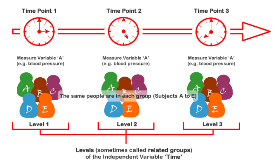
To determine whether there is a significant difference between multiple treatments or conditions within the same group of participants over time or across different variables.

Assumptions:

 Normally distributed data

 Homogeneity of variances

 Independence of observations

 Sphericity (for repeated measures)

Descriptive Statistics

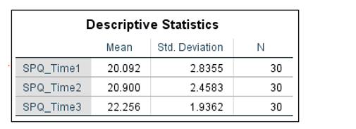
The descriptive statistics that SPSS outputs are easy enough to understand. The comparison between means (see above) gives us an idea of the direction of any possible effect. In our example, it seems as if fear of spiders increases over time, with the greatest increase (20.90 to 22.26 on the SPQ scale) occurring between year 1 (SPQ_Time2) and year 2 (SPQ_Time3). Of course, we won’t know whether these differences in the means reach significance until we look at the result of the ANOVA test.

Assumption of Sphericity

A requirement that must be met before you can trust the  p -value generated by the standard repeated-measures ANOVA is the homogeneity-of-variance-of-differences (or sphericity) assumption. For our purposes, it doesn’t matter too much what this means, we just need to know how to figure out whether the requirement has been satisfied.

SPSS tests this assumption by running Mauchly’s test of sphericity.

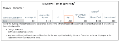
What we’re looking for here is a  p -value that’s  greater  than .05. Our  p -value is .494, which means we meet the assumption of sphericity.

Tests of Within-Subjects Effects

This is where we read off the result of the repeated-measures ANOVA test.

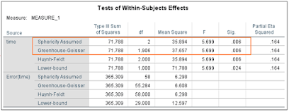
As we have just discussed, our data meets the assumption of sphericity, which means we can read our result straight from the top row (Sphericity Assumed).  The value of  F  is 5.699, which reaches significance with a  p- value of .006 (which is less than the .05 alpha level). This means there is a statistically significant difference between the means of the different levels of the within-subjects variable (time).

If our data had not met the assumption of sphericity, we would need to use one of the alternative univariate tests. You’ll notice that these produce the same value for  F , but that there is some variation in the reported degrees of freedom. In our case, there is not enough difference to alter the  p -value – Greenhouse-Geisser and Huynh-Feldt, both produce significant results  ( p  = .006).

Pairwise Comparisons

Although we know that the differences between the means of our three within-subjects levels are large enough to reach significance, we don’t yet know between which of the various pairs of means the difference is significant. This is where pairwise comparisons come into play.

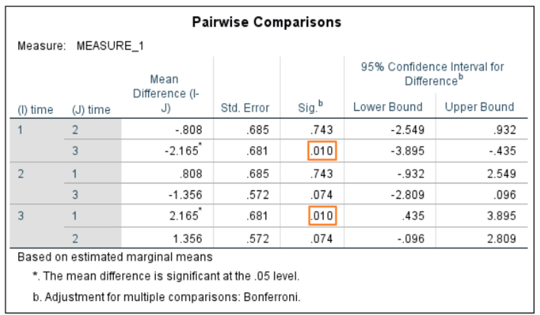
This table features three  unique  comparisons between the means for SPQ_Time1, SPQ_Time2 and SPQ_Time3. Only one of the differences reaches significance, and that’s the difference between the means for SPQ_Time1 and SPQ_Time 3 (see above). It is worth noting that SPSS is using an  adjusted  p -value  here in order to control for multiple comparisons, and that the program lets you know if a mean difference has reached significance by attaching an asterisk to the value in column 3.

Report the Result

When reporting the result it’s normal to reference both the ANOVA test and any post hoc analysis that has been done.

Thus, given our example, you could write something like:

A repeated-measures ANOVA determined that mean SPQ scores differed significantly across three time points ( F (2, 58) = 5.699,  p  = .006). A post hoc pairwise comparison using the Bonferroni correction showed an increased SPQ score between the initial assessment and follow-up assessment one year later (20.1 vs 20.9, respectively), but this was not statistically significant ( p  = .743). However, the increase in SPQ score did reach significance when comparing the initial assessment to a second follow-up assessment taken two years after the original assessment (20.1 vs 22.26, p = .010). Therefore, we can conclude that the results for the ANOVA indicate a significant time effect for untreated fear of spiders as measured on the SPQ scale.

1. Formulate the hypothesis:

    Null hypothesis (H0): There is no significant difference between the treatments/conditions.

    Alternative hypothesis (Ha): There is a significant difference between the treatments/conditions.

2. Collect data:

    Gather data on the response variable for each participant in each treatment/condition.

3. Calculate the following statistics:

    Within-subject effect (SSW): Sum of squares of deviations from the grand mean

    Between-subject effect (SSB): Sum of squares of deviations between group means

    Error effect (SSE): Sum of squares of residuals

    Mean square within (MSW): SSW divided by the degrees of freedom for within-subject effect (n-1)

    Mean square between (MSB): SSB divided by the degrees of freedom for between-subject effect (k-1)

    F-statistic: MSB divided by MSW

4. Test the hypothesis:

    Calculate the F-statistic and compare it to the critical value for the F-distribution with degrees of freedom (k-1) and (n-1)(k-1).

    If the F-statistic exceeds the critical value, reject the null hypothesis.

5. Post-hoc tests:

    If the ANOVA is significant, conduct post-hoc tests to determine which pairs of treatments/conditions are significantly different from each other.

    Commonly used tests include Tukey's HSD, Bonferroni, and Scheffé.

Advantages:

 Powerful test for detecting differences between multiple treatments/conditions.

 Controls for individual differences between participants.

Disadvantages:

 Requires balanced data with an equal number of participants in each treatment/condition.

 Assumes sphericity, which can be violated in certain designs.

ANOVA is a statistical technique used to compare the means of multiple groups when there is a single independent variable with two or more levels. In a within-subject or repeated measures design, participants are measured on multiple occasions under different conditions.

Applications in Health:

 Drug trials: Comparing the effectiveness of different drug regimens.

 Treatment efficacy: Assessing the difference in clinical outcomes before and after an intervention.

 Longitudinal studies: Monitoring the change in health parameters over time.

Consider a study investigating the effects of a new exercise program on blood pressure. Participants' blood pressure is measured at baseline (Time 1) and after 6 weeks of the program (Time 2).

ANOVA Procedure:

1. Calculate the within-subject variance: This represents the variability in participants' blood pressure over time.

2. Calculate the between-subject variance: This represents the variability in blood pressure between participants.

3. Compare the variances: Using an F-test, determine if the between-subject variance is significantly greater than the within-subject variance.

4. If there is a significant difference: Conduct post-hoc tests (e.g., paired t-tests) to determine which specific time points differ significantly.

Interpretation:

 A significant ANOVA result indicates that there is at least one significant difference in blood pressure between Time 1 and Time 2.

 Post-hoc tests can then be used to determine which specific time points show significant differences.

 Allows for comparisons of multiple conditions within the same participants.

 Reduces the impact of between-subject variability.

 Can detect changes over time or in response to interventions.

 Assumptions must be met for ANOVA to be valid, including normality of the residuals and homogeneity of variances.

 Alternative statistical techniques, such as linear mixed models, may be more appropriate for handling unbalanced or missing data.

A researcher wants to investigate the effect of three different study techniques on the test scores of students. Each student is tested on three different occasions using the different study techniques. An ANOVA for within-subject design is conducted to test whether there is a significant difference in test scores between the three techniques. 

...................................................................................................... 👉  For the data analysis, please go to my Youtube(Ads) channel to Watch Video ( Video Link ) in         Youtube Channel ( Channel Link ) and Download(Ads) video.       💗 Thanks to Subscribe(channel) and Click(channel) on bell  🔔  to get more videos!💗!! 👉 For Powerpoint presentation slide(Ads), please help to fill a short information, Please click here       ( Survey  Link ) and Download(Ads) the presentation slides from Google Drive( G_drive link )                                  💓 Thanks for your completing the  Survey 💗 👉  For more details, please contact the admin via: Tell: (+855) - 96 810 0024 Telegram:  https://t.me/sokchea_yann Facebook Page:  https://www.facebook.com/CambodiaBiostatistics/ TikTok:  https://www.tiktok.com/@sokcheayann999                                 💓 Thanks for visiting and sharing my  Facebook Page  💗 .............................................................................................................. 👉  We also provide some services as  following ​: 👉  កម្មវិធីសិក្សា : STATA for dataset restructuring, descriptive and analytical data analysis SPSS for dataset restructuring, data entry, data check, descriptive, and analytical data analysis Epi-Info for building questionnaires, data check, data entry, descriptive, and analytical data analysis Epidata-Analysis for dataset restructuring, descriptive and analytical data analysis Epi-Collect for building questionnaires, remote data entry, mapping, and data visualization Epidata-Entry for building questionnaires, data check, data entry, and data validation 👉 ចុះឈ្មោះឥលូវនេះនឹងទទួលបានតម្លៃពិសេស!🤩‼️ ................................................................................................ 👉  ព័ត៌មានបន្ថែមសូមទំនាក់ទំនងតាមរយៈ ៖ ☎️ Mobile Phone: (+855) - 96 810 0024 📳 Telegram:  https://t.me/sokchea_yann 🚩 Facebook Page:  Page 📎 Please join us:  Telegram Channel 🌎 Please visit the website Thesis Writing Skill:  Website 👬 Please follow us:  https://www.tiktok.com/@sokcheayann999 📩 Please send an email to us:  Email 🏡 Address៖ #27B, Street-271,  Street-33BT , Phsar Boeng Tumpon, Sangkat Boeng Tumpon, Khan                         Meanchey,   Phnom Penh, Cambodia.                                                    💖 Thanks for your contribution!!! 💕 ABA  Account-holder name:  Sokchea YAN ABA  Account number:  002 996 999 ABA  QR Code:   or tap on  link  below to send payment: https://pay.ababank.com/iT3dMbNKCJhp7Hgz6 ✌ Have a nice day!!! 💞

Post a comment, popular posts from this blog, what is kruskal-wallis test.

Table for statistical tests