the researchers hypothesized that being quizlet

Research Hypothesis In Psychology: Types, & Examples

Saul Mcleod, PhD

Editor-in-Chief for Simply Psychology

BSc (Hons) Psychology, MRes, PhD, University of Manchester

Saul Mcleod, PhD., is a qualified psychology teacher with over 18 years of experience in further and higher education. He has been published in peer-reviewed journals, including the Journal of Clinical Psychology.

Learn about our Editorial Process

Olivia Guy-Evans, MSc

Associate Editor for Simply Psychology

BSc (Hons) Psychology, MSc Psychology of Education

Olivia Guy-Evans is a writer and associate editor for Simply Psychology. She has previously worked in healthcare and educational sectors.

On This Page:

A research hypothesis, in its plural form “hypotheses,” is a specific, testable prediction about the anticipated results of a study, established at its outset. It is a key component of the scientific method .

Hypotheses connect theory to data and guide the research process towards expanding scientific understanding

Some key points about hypotheses:

• A hypothesis expresses an expected pattern or relationship. It connects the variables under investigation.
• It is stated in clear, precise terms before any data collection or analysis occurs. This makes the hypothesis testable.
• A hypothesis must be falsifiable. It should be possible, even if unlikely in practice, to collect data that disconfirms rather than supports the hypothesis.
• Hypotheses guide research. Scientists design studies to explicitly evaluate hypotheses about how nature works.
• For a hypothesis to be valid, it must be testable against empirical evidence. The evidence can then confirm or disprove the testable predictions.
• Hypotheses are informed by background knowledge and observation, but go beyond what is already known to propose an explanation of how or why something occurs.

Predictions typically arise from a thorough knowledge of the research literature, curiosity about real-world problems or implications, and integrating this to advance theory. They build on existing literature while providing new insight.

Types of Research Hypotheses

Alternative hypothesis.

The research hypothesis is often called the alternative or experimental hypothesis in experimental research.

It typically suggests a potential relationship between two key variables: the independent variable, which the researcher manipulates, and the dependent variable, which is measured based on those changes.

The alternative hypothesis states a relationship exists between the two variables being studied (one variable affects the other).

A hypothesis is a testable statement or prediction about the relationship between two or more variables. It is a key component of the scientific method. Some key points about hypotheses:

• Important hypotheses lead to predictions that can be tested empirically. The evidence can then confirm or disprove the testable predictions.

In summary, a hypothesis is a precise, testable statement of what researchers expect to happen in a study and why. Hypotheses connect theory to data and guide the research process towards expanding scientific understanding.

An experimental hypothesis predicts what change(s) will occur in the dependent variable when the independent variable is manipulated.

It states that the results are not due to chance and are significant in supporting the theory being investigated.

The alternative hypothesis can be directional, indicating a specific direction of the effect, or non-directional, suggesting a difference without specifying its nature. It’s what researchers aim to support or demonstrate through their study.

Null Hypothesis

The null hypothesis states no relationship exists between the two variables being studied (one variable does not affect the other). There will be no changes in the dependent variable due to manipulating the independent variable.

It states results are due to chance and are not significant in supporting the idea being investigated.

The null hypothesis, positing no effect or relationship, is a foundational contrast to the research hypothesis in scientific inquiry. It establishes a baseline for statistical testing, promoting objectivity by initiating research from a neutral stance.

Many statistical methods are tailored to test the null hypothesis, determining the likelihood of observed results if no true effect exists.

This dual-hypothesis approach provides clarity, ensuring that research intentions are explicit, and fosters consistency across scientific studies, enhancing the standardization and interpretability of research outcomes.

Nondirectional Hypothesis

A non-directional hypothesis, also known as a two-tailed hypothesis, predicts that there is a difference or relationship between two variables but does not specify the direction of this relationship.

It merely indicates that a change or effect will occur without predicting which group will have higher or lower values.

For example, “There is a difference in performance between Group A and Group B” is a non-directional hypothesis.

Directional Hypothesis

A directional (one-tailed) hypothesis predicts the nature of the effect of the independent variable on the dependent variable. It predicts in which direction the change will take place. (i.e., greater, smaller, less, more)

It specifies whether one variable is greater, lesser, or different from another, rather than just indicating that there’s a difference without specifying its nature.

For example, “Exercise increases weight loss” is a directional hypothesis.

Falsifiability

The Falsification Principle, proposed by Karl Popper , is a way of demarcating science from non-science. It suggests that for a theory or hypothesis to be considered scientific, it must be testable and irrefutable.

Falsifiability emphasizes that scientific claims shouldn’t just be confirmable but should also have the potential to be proven wrong.

It means that there should exist some potential evidence or experiment that could prove the proposition false.

However many confirming instances exist for a theory, it only takes one counter observation to falsify it. For example, the hypothesis that “all swans are white,” can be falsified by observing a black swan.

For Popper, science should attempt to disprove a theory rather than attempt to continually provide evidence to support a research hypothesis.

Can a Hypothesis be Proven?

Hypotheses make probabilistic predictions. They state the expected outcome if a particular relationship exists. However, a study result supporting a hypothesis does not definitively prove it is true.

All studies have limitations. There may be unknown confounding factors or issues that limit the certainty of conclusions. Additional studies may yield different results.

In science, hypotheses can realistically only be supported with some degree of confidence, not proven. The process of science is to incrementally accumulate evidence for and against hypothesized relationships in an ongoing pursuit of better models and explanations that best fit the empirical data. But hypotheses remain open to revision and rejection if that is where the evidence leads.

• Disproving a hypothesis is definitive. Solid disconfirmatory evidence will falsify a hypothesis and require altering or discarding it based on the evidence.
• However, confirming evidence is always open to revision. Other explanations may account for the same results, and additional or contradictory evidence may emerge over time.

We can never 100% prove the alternative hypothesis. Instead, we see if we can disprove, or reject the null hypothesis.

If we reject the null hypothesis, this doesn’t mean that our alternative hypothesis is correct but does support the alternative/experimental hypothesis.

Upon analysis of the results, an alternative hypothesis can be rejected or supported, but it can never be proven to be correct. We must avoid any reference to results proving a theory as this implies 100% certainty, and there is always a chance that evidence may exist which could refute a theory.

How to Write a Hypothesis

• Identify variables . The researcher manipulates the independent variable and the dependent variable is the measured outcome.
• Operationalized the variables being investigated . Operationalization of a hypothesis refers to the process of making the variables physically measurable or testable, e.g. if you are about to study aggression, you might count the number of punches given by participants.
• Decide on a direction for your prediction . If there is evidence in the literature to support a specific effect of the independent variable on the dependent variable, write a directional (one-tailed) hypothesis. If there are limited or ambiguous findings in the literature regarding the effect of the independent variable on the dependent variable, write a non-directional (two-tailed) hypothesis.
• Make it Testable : Ensure your hypothesis can be tested through experimentation or observation. It should be possible to prove it false (principle of falsifiability).
• Clear & concise language . A strong hypothesis is concise (typically one to two sentences long), and formulated using clear and straightforward language, ensuring it’s easily understood and testable.

Consider a hypothesis many teachers might subscribe to: students work better on Monday morning than on Friday afternoon (IV=Day, DV= Standard of work).

Now, if we decide to study this by giving the same group of students a lesson on a Monday morning and a Friday afternoon and then measuring their immediate recall of the material covered in each session, we would end up with the following:

• The alternative hypothesis states that students will recall significantly more information on a Monday morning than on a Friday afternoon.
• The null hypothesis states that there will be no significant difference in the amount recalled on a Monday morning compared to a Friday afternoon. Any difference will be due to chance or confounding factors.

More Examples

• Memory : Participants exposed to classical music during study sessions will recall more items from a list than those who studied in silence.
• Social Psychology : Individuals who frequently engage in social media use will report higher levels of perceived social isolation compared to those who use it infrequently.
• Developmental Psychology : Children who engage in regular imaginative play have better problem-solving skills than those who don’t.
• Clinical Psychology : Cognitive-behavioral therapy will be more effective in reducing symptoms of anxiety over a 6-month period compared to traditional talk therapy.
• Cognitive Psychology : Individuals who multitask between various electronic devices will have shorter attention spans on focused tasks than those who single-task.
• Health Psychology : Patients who practice mindfulness meditation will experience lower levels of chronic pain compared to those who don’t meditate.
• Organizational Psychology : Employees in open-plan offices will report higher levels of stress than those in private offices.
• Behavioral Psychology : Rats rewarded with food after pressing a lever will press it more frequently than rats who receive no reward.

What Is A Research (Scientific) Hypothesis? A plain-language explainer + examples

By:  Derek Jansen (MBA)  | Reviewed By: Dr Eunice Rautenbach | June 2020

If you’re new to the world of research, or it’s your first time writing a dissertation or thesis, you’re probably noticing that the words “research hypothesis” and “scientific hypothesis” are used quite a bit, and you’re wondering what they mean in a research context .

“Hypothesis” is one of those words that people use loosely, thinking they understand what it means. However, it has a very specific meaning within academic research. So, it’s important to understand the exact meaning before you start hypothesizing. 

Research Hypothesis 101

• What is a hypothesis ?
• What is a research hypothesis (scientific hypothesis)?
• Requirements for a research hypothesis
• Definition of a research hypothesis
• The null hypothesis

What is a hypothesis?

Let’s start with the general definition of a hypothesis (not a research hypothesis or scientific hypothesis), according to the Cambridge Dictionary:

Hypothesis: an idea or explanation for something that is based on known facts but has not yet been proved.

In other words, it’s a statement that provides an explanation for why or how something works, based on facts (or some reasonable assumptions), but that has not yet been specifically tested . For example, a hypothesis might look something like this:

Hypothesis: sleep impacts academic performance.

This statement predicts that academic performance will be influenced by the amount and/or quality of sleep a student engages in – sounds reasonable, right? It’s based on reasonable assumptions , underpinned by what we currently know about sleep and health (from the existing literature). So, loosely speaking, we could call it a hypothesis, at least by the dictionary definition.

But that’s not good enough…

Unfortunately, that’s not quite sophisticated enough to describe a research hypothesis (also sometimes called a scientific hypothesis), and it wouldn’t be acceptable in a dissertation, thesis or research paper . In the world of academic research, a statement needs a few more criteria to constitute a true research hypothesis .

What is a research hypothesis?

A research hypothesis (also called a scientific hypothesis) is a statement about the expected outcome of a study (for example, a dissertation or thesis). To constitute a quality hypothesis, the statement needs to have three attributes – specificity , clarity and testability .

Let’s take a look at these more closely.

Need a helping hand?

Hypothesis Essential #1: Specificity & Clarity

A good research hypothesis needs to be extremely clear and articulate about both what’ s being assessed (who or what variables are involved ) and the expected outcome (for example, a difference between groups, a relationship between variables, etc.).

Let’s stick with our sleepy students example and look at how this statement could be more specific and clear.

Hypothesis: Students who sleep at least 8 hours per night will, on average, achieve higher grades in standardised tests than students who sleep less than 8 hours a night.

As you can see, the statement is very specific as it identifies the variables involved (sleep hours and test grades), the parties involved (two groups of students), as well as the predicted relationship type (a positive relationship). There’s no ambiguity or uncertainty about who or what is involved in the statement, and the expected outcome is clear.

Contrast that to the original hypothesis we looked at – “Sleep impacts academic performance” – and you can see the difference. “Sleep” and “academic performance” are both comparatively vague , and there’s no indication of what the expected relationship direction is (more sleep or less sleep). As you can see, specificity and clarity are key.

Hypothesis Essential #2: Testability (Provability)

A statement must be testable to qualify as a research hypothesis. In other words, there needs to be a way to prove (or disprove) the statement. If it’s not testable, it’s not a hypothesis – simple as that.

For example, consider the hypothesis we mentioned earlier:

Hypothesis: Students who sleep at least 8 hours per night will, on average, achieve higher grades in standardised tests than students who sleep less than 8 hours a night.  

We could test this statement by undertaking a quantitative study involving two groups of students, one that gets 8 or more hours of sleep per night for a fixed period, and one that gets less. We could then compare the standardised test results for both groups to see if there’s a statistically significant difference. 

Again, if you compare this to the original hypothesis we looked at – “Sleep impacts academic performance” – you can see that it would be quite difficult to test that statement, primarily because it isn’t specific enough. How much sleep? By who? What type of academic performance?

So, remember the mantra – if you can’t test it, it’s not a hypothesis 🙂

Defining A Research Hypothesis

You’re still with us? Great! Let’s recap and pin down a clear definition of a hypothesis.

A research hypothesis (or scientific hypothesis) is a statement about an expected relationship between variables, or explanation of an occurrence, that is clear, specific and testable.

So, when you write up hypotheses for your dissertation or thesis, make sure that they meet all these criteria. If you do, you’ll not only have rock-solid hypotheses but you’ll also ensure a clear focus for your entire research project.

What about the null hypothesis?

You may have also heard the terms null hypothesis , alternative hypothesis, or H-zero thrown around. At a simple level, the null hypothesis is the counter-proposal to the original hypothesis.

For example, if the hypothesis predicts that there is a relationship between two variables (for example, sleep and academic performance), the null hypothesis would predict that there is no relationship between those variables.

At a more technical level, the null hypothesis proposes that no statistical significance exists in a set of given observations and that any differences are due to chance alone.

And there you have it – hypotheses in a nutshell. 

If you have any questions, be sure to leave a comment below and we’ll do our best to help you. If you need hands-on help developing and testing your hypotheses, consider our private coaching service , where we hold your hand through the research journey.

Psst... there’s more!

This post was based on one of our popular Research Bootcamps . If you're working on a research project, you'll definitely want to check this out ...

You Might Also Like:

16 Comments

Very useful information. I benefit more from getting more information in this regard.

Very great insight,educative and informative. Please give meet deep critics on many research data of public international Law like human rights, environment, natural resources, law of the sea etc

In a book I read a distinction is made between null, research, and alternative hypothesis. As far as I understand, alternative and research hypotheses are the same. Can you please elaborate? Best Afshin

This is a self explanatory, easy going site. I will recommend this to my friends and colleagues.

Very good definition. How can I cite your definition in my thesis? Thank you. Is nul hypothesis compulsory in a research?

It’s a counter-proposal to be proven as a rejection

Please what is the difference between alternate hypothesis and research hypothesis?

It is a very good explanation. However, it limits hypotheses to statistically tasteable ideas. What about for qualitative researches or other researches that involve quantitative data that don’t need statistical tests?

In qualitative research, one typically uses propositions, not hypotheses.

could you please elaborate it more

I’ve benefited greatly from these notes, thank you.

This is very helpful

well articulated ideas are presented here, thank you for being reliable sources of information

Excellent. Thanks for being clear and sound about the research methodology and hypothesis (quantitative research)

I have only a simple question regarding the null hypothesis. – Is the null hypothesis (Ho) known as the reversible hypothesis of the alternative hypothesis (H1? – How to test it in academic research?

this is very important note help me much more

Trackbacks/Pingbacks

• What Is Research Methodology? Simple Definition (With Examples) - Grad Coach - […] Contrasted to this, a quantitative methodology is typically used when the research aims and objectives are confirmatory in nature. For example,…

Submit a Comment Cancel reply

Your email address will not be published. Required fields are marked *

Save my name, email, and website in this browser for the next time I comment.

• Print Friendly

9 Chapter 9 Hypothesis testing

The first unit was designed to prepare you for hypothesis testing. In the first chapter we discussed the three major goals of statistics:

• Describe: connects to unit 1 with descriptive statistics and graphing
• Decide: connects to unit 1 knowing your data and hypothesis testing
• Predict: connects to hypothesis testing and unit 3

The remaining chapters will cover many different kinds of hypothesis tests connected to different inferential statistics. Needless to say, hypothesis testing is the central topic of this course. This lesson is important but that does not mean the same thing as difficult. There is a lot of new language we will learn about when conducting a hypothesis test. Some of the components of a hypothesis test are the topics we are already familiar with:

• Test statistics
• Probability
• Distribution of sample means

Hypothesis testing is an inferential procedure that uses data from a sample to draw a general conclusion about a population. It is a formal approach and a statistical method that uses sample data to evaluate hypotheses about a population. When interpreting a research question and statistical results, a natural question arises as to whether the finding could have occurred by chance. Hypothesis testing is a statistical procedure for testing whether chance (random events) is a reasonable explanation of an experimental finding. Once you have mastered the material in this lesson you will be used to solving hypothesis testing problems and the rest of the course will seem much easier. In this chapter, we will introduce the ideas behind the use of statistics to make decisions – in particular, decisions about whether a particular hypothesis is supported by the data.

Logic and Purpose of Hypothesis Testing

The statistician Ronald Fisher explained the concept of hypothesis testing with a story of a lady tasting tea. Fisher was a statistician from London and is noted as the first person to formalize the process of hypothesis testing. His elegantly simple “Lady Tasting Tea” experiment demonstrated the logic of the hypothesis test.

Figure 1. A depiction of the lady tasting tea Photo Credit

Fisher would often have afternoon tea during his studies. He usually took tea with a woman who claimed to be a tea expert. In particular, she told Fisher that she could tell which was poured first in the teacup, the milk or the tea, simply by tasting the cup. Fisher, being a scientist, decided to put this rather bizarre claim to the test. The lady accepted his challenge. Fisher brought her 8 cups of tea in succession; 4 cups would be prepared with the milk added first, and 4 with the tea added first. The cups would be presented in a random order unknown to the lady.

The lady would take a sip of each cup as it was presented and report which ingredient she believed was poured first. Using the laws of probability, Fisher determined the chances of her guessing all 8 cups correctly was 1/70, or about 1.4%. In other words, if the lady was indeed guessing there was a 1.4% chance of her getting all 8 cups correct. On the day of the experiment, Fisher had 8 cups prepared just as he had requested. The lady drank each cup and made her decisions for each one.

After the experiment, it was revealed that the lady got all 8 cups correct! Remember, had she been truly guessing, the chance of getting this result was 1.4%. Since this probability was so low , Fisher instead concluded that the lady could indeed differentiate between the milk or the tea being poured first. Fisher’s original hypothesis that she was just guessing was demonstrated to be false and was therefore rejected. The alternative hypothesis, that the lady could truly tell the cups apart, was then accepted as true.

This story demonstrates many components of hypothesis testing in a very simple way. For example, Fisher started with a hypothesis that the lady was guessing. He then determined that if she was indeed guessing, the probability of guessing all 8 right was very small, just 1.4%. Since that probability was so tiny, when she did get all 8 cups right, Fisher determined it was extremely unlikely she was guessing. A more reasonable conclusion was that the lady had the skill to tell the cups apart.

In hypothesis testing, we will always set up a particular hypothesis that we want to demonstrate to be true. We then use probability to determine the likelihood of our hypothesis is correct. If it appears our original hypothesis was wrong, we reject it and accept the alternative hypothesis. The alternative hypothesis is usually the opposite of our original hypothesis. In Fisher’s case, his original hypothesis was that the lady was guessing. His alternative hypothesis was the lady was not guessing.

This result does not prove that he does; it could be he was just lucky and guessed right 13 out of 16 times. But how plausible is the explanation that he was just lucky? To assess its plausibility, we determine the probability that someone who was just guessing would be correct 13/16 times or more. This probability can be computed to be 0.0106. This is a pretty low probability, and therefore someone would have to be very lucky to be correct 13 or more times out of 16 if they were just guessing. A low probability gives us more confidence there is evidence Bond can tell whether the drink was shaken or stirred. There is also still a chance that Mr. Bond was very lucky (more on this later!). The hypothesis that he was guessing is not proven false, but considerable doubt is cast on it. Therefore, there is strong evidence that Mr. Bond can tell whether a drink was shaken or stirred.

You may notice some patterns here:

• We have 2 hypotheses: the original (researcher prediction) and the alternative
• We collect data
• We determine how likley or unlikely the original hypothesis is to occur based on probability.
• We determine if we have enough evidence to support the original hypothesis and draw conclusions.

Now let’s being in some specific terminology:

Null hypothesis : In general, the null hypothesis, written H 0 (“H-naught”), is the idea that nothing is going on: there is no effect of our treatment, no relation between our variables, and no difference in our sample mean from what we expected about the population mean. The null hypothesis indicates that an apparent effect is due to chance. This is always our baseline starting assumption, and it is what we (typically) seek to reject . For mathematical notation, one uses =).

Alternative hypothesis : If the null hypothesis is rejected, then we will need some other explanation, which we call the alternative hypothesis, H A or H 1 . The alternative hypothesis is simply the reverse of the null hypothesis. Thus, our alternative hypothesis is the mathematical way of stating our research question.  In general, the alternative hypothesis (also called the research hypothesis)is there is an effect of treatment, the relation between variables, or differences in a sample mean compared to a population mean. The alternative hypothesis essentially shows evidence the findings are not due to chance.  It is also called the research hypothesis as this is the most common outcome a researcher is looking for: evidence of change, differences, or relationships. There are three options for setting up the alternative hypothesis, depending on where we expect the difference to lie. The alternative hypothesis always involves some kind of inequality (≠not equal, >, or <).

• If we expect a specific direction of change/differences/relationships, which we call a directional hypothesis , then our alternative hypothesis takes the form based on the research question itself.  One would expect a decrease in depression from taking an anti-depressant as a specific directional hypothesis.  Or the direction could be larger, where for example, one might expect an increase in exam scores after completing a student success exam preparation module.  The directional hypothesis (2 directions) makes up 2 of the 3 alternative hypothesis options.  The other alternative is to state there are differences/changes, or a relationship but not predict the direction.  We use a non-directional alternative hypothesis  (typically see ≠ for mathematical notation).

Probability value (p-value) : the probability of a certain outcome assuming a certain state of the world. In statistics, it is conventional to refer to possible states of the world as hypotheses since they are hypothesized states of the world. Using this terminology, the probability value is the probability of an outcome given the hypothesis. It is not the probability of the hypothesis given the outcome. It is very important to understand precisely what the probability values mean. In the James Bond example, the computed probability of 0.0106 is the probability he would be correct on 13 or more taste tests (out of 16) if he were just guessing. It is easy to mistake this probability of 0.0106 as the probability he cannot tell the difference. This is not at all what it means. The probability of 0.0106 is the probability of a certain outcome (13 or more out of 16) assuming a certain state of the world (James Bond was only guessing).

A low probability value casts doubt on the null hypothesis. How low must the probability value be in order to conclude that the null hypothesis is false? Although there is clearly no right or wrong answer to this question, it is conventional to conclude the null hypothesis is false if the probability value is less than 0.05 (p < .05). More conservative researchers conclude the null hypothesis is false only if the probability value is less than 0.01 (p<.01). When a researcher concludes that the null hypothesis is false, the researcher is said to have rejected the null hypothesis. The probability value below which the null hypothesis is rejected is called the α level or simply α (“alpha”). It is also called the significance level . If α is not explicitly specified, assume that α = 0.05.

Decision-making is part of the process and we have some language that goes along with that. Importantly, null hypothesis testing operates under the assumption that the null hypothesis is true unless the evidence shows otherwise. We (typically) seek to reject the null hypothesis, giving us evidence to support the alternative hypothesis .  If the probability of the outcome given the hypothesis is sufficiently low, we have evidence that the null hypothesis is false. Note that all probability calculations for all hypothesis tests center on the null hypothesis. In the James Bond example, the null hypothesis is that he cannot tell the difference between shaken and stirred martinis. The probability value is low that one is able to identify 13 of 16 martinis as shaken or stirred (0.0106), thus providing evidence that he can tell the difference. Note that we have not computed the probability that he can tell the difference.

The specific type of hypothesis testing reviewed is specifically known as null hypothesis statistical testing (NHST). We can break the process of null hypothesis testing down into a number of steps a researcher would use.

• Formulate a hypothesis that embodies our prediction ( before seeing the data )
• Specify null and alternative hypotheses
• Collect some data relevant to the hypothesis
• Compute a test statistic
• Identify the criteria probability (or compute the probability of the observed value of that statistic) assuming that the null hypothesis is true
• Drawing conclusions. Assess the “statistical significance” of the result

Steps in hypothesis testing

Step 1: formulate a hypothesis of interest.

The researchers hypothesized that physicians spend less time with obese patients. The researchers hypothesis derived from an identified population. In creating a research hypothesis, we also have to decide whether we want to test a directional or non-directional hypotheses. Researchers typically will select a non-directional hypothesis for a more conservative approach, particularly when the outcome is unknown (more about why this is later).

Step 2: Specify the null and alternative hypotheses

Can you set up the null and alternative hypotheses for the Physician’s Reaction Experiment?

Step 3: Determine the alpha level.

For this course, alpha will be given to you as .05 or .01.  Researchers will decide on alpha and then determine the associated test statistic based from the sample. Researchers in the Physician Reaction study might set the alpha at .05 and identify the test statistics associated with the .05 for the sample size.  Researchers might take extra precautions to be more confident in their findings (more on this later).

Step 4: Collect some data

For this course, the data will be given to you.  Researchers collect the data and then start to summarize it using descriptive statistics. The mean time physicians reported that they would spend with obese patients was 24.7 minutes as compared to a mean of 31.4 minutes for normal-weight patients.

Step 5: Compute a test statistic

We next want to use the data to compute a statistic that will ultimately let us decide whether the null hypothesis is rejected or not. We can think of the test statistic as providing a measure of the size of the effect compared to the variability in the data. In general, this test statistic will have a probability distribution associated with it, because that allows us to determine how likely our observed value of the statistic is under the null hypothesis.

To assess the plausibility of the hypothesis that the difference in mean times is due to chance, we compute the probability of getting a difference as large or larger than the observed difference (31.4 – 24.7 = 6.7 minutes) if the difference were, in fact, due solely to chance.

Step 6: Determine the probability of the observed result under the null hypothesis 

Using methods presented in later chapters, this probability associated with the observed differences between the two groups for the Physician’s Reaction was computed to be 0.0057. Since this is such a low probability, we have confidence that the difference in times is due to the patient’s weight (obese or not) (and is not due to chance). We can then reject the null hypothesis (there are no differences or differences seen are due to chance).

Keep in mind that the null hypothesis is typically the opposite of the researcher’s hypothesis. In the Physicians’ Reactions study, the researchers hypothesized that physicians would expect to spend less time with obese patients. The null hypothesis that the two types of patients are treated identically as part of the researcher’s control of other variables. If the null hypothesis were true, a difference as large or larger than the sample difference of 6.7 minutes would be very unlikely to occur. Therefore, the researchers rejected the null hypothesis of no difference and concluded that in the population, physicians intend to spend less time with obese patients.

This is the step where NHST starts to violate our intuition. Rather than determining the likelihood that the null hypothesis is true given the data, we instead determine the likelihood under the null hypothesis of observing a statistic at least as extreme as one that we have observed — because we started out by assuming that the null hypothesis is true! To do this, we need to know the expected probability distribution for the statistic under the null hypothesis, so that we can ask how likely the result would be under that distribution. This will be determined from a table we use for reference or calculated in a statistical analysis program. Note that when I say “how likely the result would be”, what I really mean is “how likely the observed result or one more extreme would be”. We need to add this caveat as we are trying to determine how weird our result would be if the null hypothesis were true, and any result that is more extreme will be even more weird, so we want to count all of those weirder possibilities when we compute the probability of our result under the null hypothesis.

Let’s review some considerations for Null hypothesis statistical testing (NHST)!

Null hypothesis statistical testing (NHST) is commonly used in many fields. If you pick up almost any scientific or biomedical research publication, you will see NHST being used to test hypotheses, and in their introductory psychology textbook, Gerrig & Zimbardo (2002) referred to NHST as the “backbone of psychological research”. Thus, learning how to use and interpret the results from hypothesis testing is essential to understand the results from many fields of research.

It is also important for you to know, however, that NHST is flawed, and that many statisticians and researchers think that it has been the cause of serious problems in science, which we will discuss in further in this unit. NHST is also widely misunderstood, largely because it violates our intuitions about how statistical hypothesis testing should work. Let’s look at an example to see this.

There is great interest in the use of body-worn cameras by police officers, which are thought to reduce the use of force and improve officer behavior. However, in order to establish this we need experimental evidence, and it has become increasingly common for governments to use randomized controlled trials to test such ideas. A randomized controlled trial of the effectiveness of body-worn cameras was performed by the Washington, DC government and DC Metropolitan Police Department in 2015-2016. Officers were randomly assigned to wear a body-worn camera or not, and their behavior was then tracked over time to determine whether the cameras resulted in less use of force and fewer civilian complaints about officer behavior.

Before we get to the results, let’s ask how you would think the statistical analysis might work. Let’s say we want to specifically test the hypothesis of whether the use of force is decreased by the wearing of cameras. The randomized controlled trial provides us with the data to test the hypothesis – namely, the rates of use of force by officers assigned to either the camera or control groups. The next obvious step is to look at the data and determine whether they provide convincing evidence for or against this hypothesis. That is: What is the likelihood that body-worn cameras reduce the use of force, given the data and everything else we know?

It turns out that this is not how null hypothesis testing works. Instead, we first take our hypothesis of interest (i.e. that body-worn cameras reduce use of force), and flip it on its head, creating a null hypothesis – in this case, the null hypothesis would be that cameras do not reduce use of force. Importantly, we then assume that the null hypothesis is true. We then look at the data, and determine how likely the data would be if the null hypothesis were true. If the data are sufficiently unlikely under the null hypothesis that we can reject the null in favor of the alternative hypothesis which is our hypothesis of interest. If there is not sufficient evidence to reject the null, then we say that we retain (or “fail to reject”) the null, sticking with our initial assumption that the null is true.

Understanding some of the concepts of NHST, particularly the notorious “p-value”, is invariably challenging the first time one encounters them, because they are so counter-intuitive. As we will see later, there are other approaches that provide a much more intuitive way to address hypothesis testing (but have their own complexities).

Step 7: Assess the “statistical significance” of the result. Draw conclusions.

The next step is to determine whether the p-value that results from the previous step is small enough that we are willing to reject the null hypothesis and conclude instead that the alternative is true. In the Physicians Reactions study, the probability value is 0.0057. Therefore, the effect of obesity is statistically significant and the null hypothesis that obesity makes no difference is rejected. It is very important to keep in mind that statistical significance means only that the null hypothesis of exactly no effect is rejected; it does not mean that the effect is important, which is what “significant” usually means. When an effect is significant, you can have confidence the effect is not exactly zero. Finding that an effect is significant does not tell you about how large or important the effect is.

How much evidence do we require and what considerations are needed to better understand the significance of the findings? This is one of the most controversial questions in statistics, in part because it requires a subjective judgment – there is no “correct” answer.

What does a statistically significant result mean?

There is a great deal of confusion about what p-values actually mean (Gigerenzer, 2004). Let’s say that we do an experiment comparing the means between conditions, and we find a difference with a p-value of .01. There are a number of possible interpretations that one might entertain.

Does it mean that the probability of the null hypothesis being true is .01? No. Remember that in null hypothesis testing, the p-value is the probability of the data given the null hypothesis. It does not warrant conclusions about the probability of the null hypothesis given the data.

Does it mean that the probability that you are making the wrong decision is .01? No. Remember as above that p-values are probabilities of data under the null, not probabilities of hypotheses.

Does it mean that if you ran the study again, you would obtain the same result 99% of the time? No. The p-value is a statement about the likelihood of a particular dataset under the null; it does not allow us to make inferences about the likelihood of future events such as replication.

Does it mean that you have found a practially important effect? No. There is an essential distinction between statistical significance and practical significance . As an example, let’s say that we performed a randomized controlled trial to examine the effect of a particular diet on body weight, and we find a statistically significant effect at p<.05. What this doesn’t tell us is how much weight was actually lost, which we refer to as the effect size (to be discussed in more detail). If we think about a study of weight loss, then we probably don’t think that the loss of one ounce (i.e. the weight of a few potato chips) is practically significant. Let’s look at our ability to detect a significant difference of 1 ounce as the sample size increases.

A statistically significant result is not necessarily a strong one. Even a very weak result can be statistically significant if it is based on a large enough sample. This is why it is important to distinguish between the statistical significance of a result and the practical significance of that result. Practical significance refers to the importance or usefulness of the result in some real-world context and is often referred to as the effect size .

Many differences are statistically significant—and may even be interesting for purely scientific reasons—but they are not practically significant. In clinical practice, this same concept is often referred to as “clinical significance.” For example, a study on a new treatment for social phobia might show that it produces a statistically significant positive effect. Yet this effect still might not be strong enough to justify the time, effort, and other costs of putting it into practice—especially if easier and cheaper treatments that work almost as well already exist. Although statistically significant, this result would be said to lack practical or clinical significance.

Be aware that the term effect size can be misleading because it suggests a causal relationship—that the difference between the two means is an “effect” of being in one group or condition as opposed to another. In other words, simply calling the difference an “effect size” does not make the relationship a causal one.

Figure 1 shows how the proportion of significant results increases as the sample size increases, such that with a very large sample size (about 262,000 total subjects), we will find a significant result in more than 90% of studies when there is a 1 ounce difference in weight loss between the diets. While these are statistically significant, most physicians would not consider a weight loss of one ounce to be practically or clinically significant. We will explore this relationship in more detail when we return to the concept of statistical power in Chapter X, but it should already be clear from this example that statistical significance is not necessarily indicative of practical significance.

Figure 1: The proportion of significant results for a very small change (1 ounce, which is about .001 standard deviations) as a function of sample size.

Challenges with using p-values

Historically, the most common answer to this question has been that we should reject the null hypothesis if the p-value is less than 0.05. This comes from the writings of Ronald Fisher, who has been referred to as “the single most important figure in 20th century statistics” (Efron, 1998 ) :

“If P is between .1 and .9 there is certainly no reason to suspect the hypothesis tested. If it is below .02 it is strongly indicated that the hypothesis fails to account for the whole of the facts. We shall not often be astray if we draw a conventional line at .05 … it is convenient to draw the line at about the level at which we can say: Either there is something in the treatment, or a coincidence has occurred such as does not occur more than once in twenty trials” (Fisher, 1925 )

Fisher never intended p<0.05p < 0.05 to be a fixed rule:

“no scientific worker has a fixed level of significance at which from year to year, and in all circumstances, he rejects hypotheses; he rather gives his mind to each particular case in the light of his evidence and his ideas” (Fisher, 1956 )

Instead, it is likely that p < .05 became a ritual due to the reliance upon tables of p-values that were used before computing made it easy to compute p values for arbitrary values of a statistic. All of the tables had an entry for 0.05, making it easy to determine whether one’s statistic exceeded the value needed to reach that level of significance. Although we use tables in this class, statistical software examines the specific probability value for the calculated statistic.

Assessing Error Rate: Type I and Type II Error

Although there are challenges with p-values for decision making, we will examine a way we can think about hypothesis testing in terms of its error rate.  This was proposed by Jerzy Neyman and Egon Pearson:

“no test based upon a theory of probability can by itself provide any valuable evidence of the truth or falsehood of a hypothesis. But we may look at the purpose of tests from another viewpoint. Without hoping to know whether each separate hypothesis is true or false, we may search for rules to govern our behaviour with regard to them, in following which we insure that, in the long run of experience, we shall not often be wrong” (Neyman & Pearson, 1933 )

That is: We can’t know which specific decisions are right or wrong, but if we follow the rules, we can at least know how often our decisions will be wrong in the long run.

To understand the decision-making framework that Neyman and Pearson developed, we first need to discuss statistical decision-making in terms of the kinds of outcomes that can occur. There are two possible states of reality (H0 is true, or H0 is false), and two possible decisions (reject H0, or retain H0). There are two ways in which we can make a correct decision:

• We can reject H0 when it is false (in the language of signal detection theory, we call this a hit )
• We can retain H0 when it is true (somewhat confusingly in this context, this is called a correct rejection )

There are also two kinds of errors we can make:

• We can reject H0 when it is actually true (we call this a false alarm , or Type I error ), Type I error  means that we have concluded that there is a relationship in the population when in fact there is not. Type I errors occur because even when there is no relationship in the population, sampling error alone will occasionally produce an extreme result.
• We can retain H0 when it is actually false (we call this a miss , or Type II error ). Type II error  means that we have concluded that there is no relationship in the population when in fact there is.

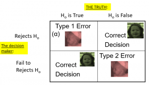
Summing up, when you perform a hypothesis test, there are four possible outcomes depending on the actual truth (or falseness) of the null hypothesis H0 and the decision to reject or not. The outcomes are summarized in the following table:

Table 1. The four possible outcomes in hypothesis testing.

• The decision is not to reject H0 when H0 is true (correct decision).
• The decision is to reject H0 when H0 is true (incorrect decision known as a Type I error ).
• The decision is not to reject H0 when, in fact, H0 is false (incorrect decision known as a Type II error ).
• The decision is to reject H0 when H0 is false ( correct decision ).

Neyman and Pearson coined two terms to describe the probability of these two types of errors in the long run:

• P(Type I error) = αalpha
• P(Type II error) = βbeta

That is, if we set αalpha to .05, then in the long run we should make a Type I error 5% of the time. The 𝞪 (alpha) , is associated with the p-value for the level of significance. Again it’s common to set αalpha as .05. In fact, when the null hypothesis is true and α is .05, we will mistakenly reject the null hypothesis 5% of the time. (This is why α is sometimes referred to as the “Type I error rate.”) In principle, it is possible to reduce the chance of a Type I error by setting α to something less than .05. Setting it to .01, for example, would mean that if the null hypothesis is true, then there is only a 1% chance of mistakenly rejecting it. But making it harder to reject true null hypotheses also makes it harder to reject false ones and therefore increases the chance of a Type II error.

In practice, Type II errors occur primarily because the research design lacks adequate statistical power to detect the relationship (e.g., the sample is too small).  Statistical power is the complement of Type II error. We will have more to say about statistical power shortly. The standard value for an acceptable level of β (beta) is .2 – that is, we are willing to accept that 20% of the time we will fail to detect a true effect when it truly exists. It is possible to reduce the chance of a Type II error by setting α to something greater than .05 (e.g., .10). But making it easier to reject false null hypotheses also makes it easier to reject true ones and therefore increases the chance of a Type I error. This provides some insight into why the convention is to set α to .05. There is some agreement among researchers that level of α keeps the rates of both Type I and Type II errors at acceptable levels.

The possibility of committing Type I and Type II errors has several important implications for interpreting the results of our own and others’ research. One is that we should be cautious about interpreting the results of any individual study because there is a chance that it reflects a Type I or Type II error. This is why researchers consider it important to replicate their studies. Each time researchers replicate a study and find a similar result, they rightly become more confident that the result represents a real phenomenon and not just a Type I or Type II error.

Test Statistic Assumptions

Last consideration we will revisit with each test statistic (e.g., t-test, z-test and ANOVA) in the coming chapters.  There are four main assumptions. These assumptions are often taken for granted in using prescribed data for the course.  In the real world, these assumptions would need to be examined, often tested using statistical software.

• Assumption of random sampling. A sample is random when each person (or animal) point in your population has an equal chance of being included in the sample; therefore selection of any individual happens by chance, rather than by choice. This reduces the chance that differences in materials, characteristics or conditions may bias results. Remember that random samples are more likely to be representative of the population so researchers can be more confident interpreting the results. Note: there is no test that statistical software can perform which assures random sampling has occurred but following good sampling techniques helps to ensure your samples are random.
• Assumption of Independence. Statistical independence is a critical assumption for many statistical tests including the 2-sample t-test and ANOVA. It is assumed that observations are independent of each other often but often this assumption. Is not met. Independence means the value of one observation does not influence or affect the value of other observations. Independent data items are not connected with one another in any way (unless you account for it in your study). Even the smallest dependence in your data can turn into heavily biased results (which may be undetectable) if you violate this assumption. Note: there is no test statistical software can perform that assures independence of the data because this should be addressed during the research planning phase. Using a non-parametric test is often recommended if a researcher is concerned this assumption has been violated.
• Assumption of Normality. Normality assumes that the continuous variables (dependent variable) used in the analysis are normally distributed. Normal distributions are symmetric around the center (the mean) and form a bell-shaped distribution. Normality is violated when sample data are skewed. With large enough sample sizes (n > 30) the violation of the normality assumption should not cause major problems (remember the central limit theorem) but there is a feature in most statistical software that can alert researchers to an assumption violation.
• Assumption of Equal Variance. Variance refers to the spread or of scores from the mean. Many statistical tests assume that although different samples can come from populations with different means, they have the same variance. Equality of variance (i.e., homogeneity of variance) is violated when variances across different groups or samples are significantly different. Note: there is a feature in most statistical software to test for this.

We will use 4 main steps for hypothesis testing:

• Usually the hypotheses concern population parameters and predict the characteristics that a sample should have
• Null: Null hypothesis (H0) states that there is no difference, no effect or no change between population means and sample means. There is no difference.
• Alternative: Alternative hypothesis (H1 or HA) states that there is a difference or a change between the population and sample. It is the opposite of the null hypothesis.
• Set criteria for a decision. In this step we must determine the boundary of our distribution at which the null hypothesis will be rejected. Researchers usually use either a 5% (.05) cutoff or 1% (.01) critical boundary. Recall from our earlier story about Ronald Fisher that the lower the probability the more confident the was that the Tea Lady was not guessing.  We will apply this to z in the next chapter.
• Compare sample and population to decide if the hypothesis has support
• When a researcher uses hypothesis testing, the individual is making a decision about whether the data collected is sufficient to state that the population parameters are significantly different.

Further considerations

The probability value is the probability of a result as extreme or more extreme given that the null hypothesis is true. It is the probability of the data given the null hypothesis. It is not the probability that the null hypothesis is false.

A low probability value indicates that the sample outcome (or one more extreme) would be very unlikely if the null hypothesis were true. We will learn more about assessing effect size later in this unit.

3.  A non-significant outcome means that the data do not conclusively demonstrate that the null hypothesis is false. There is always a chance of error and 4 outcomes associated with hypothesis testing.

• It is important to take into account the assumptions for each test statistic.

Learning objectives

Having read the chapter, you should be able to:

• Identify the components of a hypothesis test, including the parameter of interest, the null and alternative hypotheses, and the test statistic.
• State the hypotheses and identify appropriate critical areas depending on how hypotheses are set up.
• Describe the proper interpretations of a p-value as well as common misinterpretations.
• Distinguish between the two types of error in hypothesis testing, and the factors that determine them.
• Describe the main criticisms of null hypothesis statistical testing
• Identify the purpose of effect size and power.

Exercises – Ch. 9

• In your own words, explain what the null hypothesis is.
• What are Type I and Type II Errors?
• Why do we phrase null and alternative hypotheses with population parameters and not sample means?
• If our null hypothesis is “H0: μ = 40”, what are the three possible alternative hypotheses?
• Why do we state our hypotheses and decision criteria before we collect our data?
• When and why do you calculate an effect size?

Answers to Odd- Numbered Exercises – Ch. 9

1. Your answer should include mention of the baseline assumption of no difference between the sample and the population.

3. Alpha is the significance level. It is the criteria we use when decided to reject or fail to reject the null hypothesis, corresponding to a given proportion of the area under the normal distribution and a probability of finding extreme scores assuming the null hypothesis is true.

5. μ > 40; μ < 40; μ ≠ 40

7. We calculate effect size to determine the strength of the finding.  Effect size should always be calculated when the we have rejected the null hypothesis.  Effect size can be calculated for non-significant findings as a possible indicator of Type II error.

Introduction to Statistics for Psychology Copyright © 2021 by Alisa Beyer is licensed under a Creative Commons Attribution-NonCommercial-ShareAlike 4.0 International License , except where otherwise noted.

Share This Book

• Bipolar Disorder
• Therapy Center
• When To See a Therapist
• Types of Therapy
• Best Online Therapy
• Best Couples Therapy
• Best Family Therapy
• Managing Stress
• Sleep and Dreaming
• Understanding Emotions
• Self-Improvement
• Healthy Relationships
• Student Resources
• Personality Types
• Guided Meditations
• Verywell Mind Insights
• 2024 Verywell Mind 25
• Mental Health in the Classroom
• Editorial Process
• Meet Our Review Board
• Crisis Support

How to Write a Great Hypothesis

Hypothesis Definition, Format, Examples, and Tips

Kendra Cherry, MS, is a psychosocial rehabilitation specialist, psychology educator, and author of the "Everything Psychology Book."

Amy Morin, LCSW, is a psychotherapist and international bestselling author. Her books, including "13 Things Mentally Strong People Don't Do," have been translated into more than 40 languages. Her TEDx talk,  "The Secret of Becoming Mentally Strong," is one of the most viewed talks of all time.

Verywell / Alex Dos Diaz

• The Scientific Method

Hypothesis Format

Falsifiability of a hypothesis.

• Operationalization

Hypothesis Types

Hypotheses examples.

• Collecting Data

A hypothesis is a tentative statement about the relationship between two or more variables. It is a specific, testable prediction about what you expect to happen in a study. It is a preliminary answer to your question that helps guide the research process.

Consider a study designed to examine the relationship between sleep deprivation and test performance. The hypothesis might be: "This study is designed to assess the hypothesis that sleep-deprived people will perform worse on a test than individuals who are not sleep-deprived."

At a Glance

A hypothesis is crucial to scientific research because it offers a clear direction for what the researchers are looking to find. This allows them to design experiments to test their predictions and add to our scientific knowledge about the world. This article explores how a hypothesis is used in psychology research, how to write a good hypothesis, and the different types of hypotheses you might use.

The Hypothesis in the Scientific Method

In the scientific method , whether it involves research in psychology, biology, or some other area, a hypothesis represents what the researchers think will happen in an experiment. The scientific method involves the following steps:

• Forming a question
• Performing background research
• Creating a hypothesis
• Designing an experiment
• Collecting data
• Analyzing the results
• Drawing conclusions
• Communicating the results

The hypothesis is a prediction, but it involves more than a guess. Most of the time, the hypothesis begins with a question which is then explored through background research. At this point, researchers then begin to develop a testable hypothesis.

Unless you are creating an exploratory study, your hypothesis should always explain what you  expect  to happen.

In a study exploring the effects of a particular drug, the hypothesis might be that researchers expect the drug to have some type of effect on the symptoms of a specific illness. In psychology, the hypothesis might focus on how a certain aspect of the environment might influence a particular behavior.

Remember, a hypothesis does not have to be correct. While the hypothesis predicts what the researchers expect to see, the goal of the research is to determine whether this guess is right or wrong. When conducting an experiment, researchers might explore numerous factors to determine which ones might contribute to the ultimate outcome.

In many cases, researchers may find that the results of an experiment  do not  support the original hypothesis. When writing up these results, the researchers might suggest other options that should be explored in future studies.

In many cases, researchers might draw a hypothesis from a specific theory or build on previous research. For example, prior research has shown that stress can impact the immune system. So a researcher might hypothesize: "People with high-stress levels will be more likely to contract a common cold after being exposed to the virus than people who have low-stress levels."

In other instances, researchers might look at commonly held beliefs or folk wisdom. "Birds of a feather flock together" is one example of folk adage that a psychologist might try to investigate. The researcher might pose a specific hypothesis that "People tend to select romantic partners who are similar to them in interests and educational level."

Elements of a Good Hypothesis

So how do you write a good hypothesis? When trying to come up with a hypothesis for your research or experiments, ask yourself the following questions:

• Is your hypothesis based on your research on a topic?
• Can your hypothesis be tested?
• Does your hypothesis include independent and dependent variables?

Before you come up with a specific hypothesis, spend some time doing background research. Once you have completed a literature review, start thinking about potential questions you still have. Pay attention to the discussion section in the  journal articles you read . Many authors will suggest questions that still need to be explored.

How to Formulate a Good Hypothesis

To form a hypothesis, you should take these steps:

• Collect as many observations about a topic or problem as you can.
• Evaluate these observations and look for possible causes of the problem.
• Create a list of possible explanations that you might want to explore.
• After you have developed some possible hypotheses, think of ways that you could confirm or disprove each hypothesis through experimentation. This is known as falsifiability.

In the scientific method ,  falsifiability is an important part of any valid hypothesis. In order to test a claim scientifically, it must be possible that the claim could be proven false.

Students sometimes confuse the idea of falsifiability with the idea that it means that something is false, which is not the case. What falsifiability means is that  if  something was false, then it is possible to demonstrate that it is false.

One of the hallmarks of pseudoscience is that it makes claims that cannot be refuted or proven false.

The Importance of Operational Definitions

A variable is a factor or element that can be changed and manipulated in ways that are observable and measurable. However, the researcher must also define how the variable will be manipulated and measured in the study.

Operational definitions are specific definitions for all relevant factors in a study. This process helps make vague or ambiguous concepts detailed and measurable.

For example, a researcher might operationally define the variable " test anxiety " as the results of a self-report measure of anxiety experienced during an exam. A "study habits" variable might be defined by the amount of studying that actually occurs as measured by time.

These precise descriptions are important because many things can be measured in various ways. Clearly defining these variables and how they are measured helps ensure that other researchers can replicate your results.

Replicability

One of the basic principles of any type of scientific research is that the results must be replicable.

Replication means repeating an experiment in the same way to produce the same results. By clearly detailing the specifics of how the variables were measured and manipulated, other researchers can better understand the results and repeat the study if needed.

Some variables are more difficult than others to define. For example, how would you operationally define a variable such as aggression ? For obvious ethical reasons, researchers cannot create a situation in which a person behaves aggressively toward others.

To measure this variable, the researcher must devise a measurement that assesses aggressive behavior without harming others. The researcher might utilize a simulated task to measure aggressiveness in this situation.

Hypothesis Checklist

• Does your hypothesis focus on something that you can actually test?
• Does your hypothesis include both an independent and dependent variable?
• Can you manipulate the variables?
• Can your hypothesis be tested without violating ethical standards?

The hypothesis you use will depend on what you are investigating and hoping to find. Some of the main types of hypotheses that you might use include:

• Simple hypothesis : This type of hypothesis suggests there is a relationship between one independent variable and one dependent variable.
• Complex hypothesis : This type suggests a relationship between three or more variables, such as two independent and dependent variables.
• Null hypothesis : This hypothesis suggests no relationship exists between two or more variables.
• Alternative hypothesis : This hypothesis states the opposite of the null hypothesis.
• Statistical hypothesis : This hypothesis uses statistical analysis to evaluate a representative population sample and then generalizes the findings to the larger group.
• Logical hypothesis : This hypothesis assumes a relationship between variables without collecting data or evidence.

A hypothesis often follows a basic format of "If {this happens} then {this will happen}." One way to structure your hypothesis is to describe what will happen to the  dependent variable  if you change the  independent variable .

The basic format might be: "If {these changes are made to a certain independent variable}, then we will observe {a change in a specific dependent variable}."

A few examples of simple hypotheses:

• "Students who eat breakfast will perform better on a math exam than students who do not eat breakfast."
• "Students who experience test anxiety before an English exam will get lower scores than students who do not experience test anxiety."​
• "Motorists who talk on the phone while driving will be more likely to make errors on a driving course than those who do not talk on the phone."
• "Children who receive a new reading intervention will have higher reading scores than students who do not receive the intervention."

Examples of a complex hypothesis include:

• "People with high-sugar diets and sedentary activity levels are more likely to develop depression."
• "Younger people who are regularly exposed to green, outdoor areas have better subjective well-being than older adults who have limited exposure to green spaces."

Examples of a null hypothesis include:

• "There is no difference in anxiety levels between people who take St. John's wort supplements and those who do not."
• "There is no difference in scores on a memory recall task between children and adults."
• "There is no difference in aggression levels between children who play first-person shooter games and those who do not."

Examples of an alternative hypothesis:

• "People who take St. John's wort supplements will have less anxiety than those who do not."
• "Adults will perform better on a memory task than children."
• "Children who play first-person shooter games will show higher levels of aggression than children who do not." 

Collecting Data on Your Hypothesis

Once a researcher has formed a testable hypothesis, the next step is to select a research design and start collecting data. The research method depends largely on exactly what they are studying. There are two basic types of research methods: descriptive research and experimental research.

Descriptive Research Methods

Descriptive research such as  case studies ,  naturalistic observations , and surveys are often used when  conducting an experiment is difficult or impossible. These methods are best used to describe different aspects of a behavior or psychological phenomenon.

Once a researcher has collected data using descriptive methods, a  correlational study  can examine how the variables are related. This research method might be used to investigate a hypothesis that is difficult to test experimentally.

Experimental Research Methods

Experimental methods  are used to demonstrate causal relationships between variables. In an experiment, the researcher systematically manipulates a variable of interest (known as the independent variable) and measures the effect on another variable (known as the dependent variable).

Unlike correlational studies, which can only be used to determine if there is a relationship between two variables, experimental methods can be used to determine the actual nature of the relationship—whether changes in one variable actually  cause  another to change.

The hypothesis is a critical part of any scientific exploration. It represents what researchers expect to find in a study or experiment. In situations where the hypothesis is unsupported by the research, the research still has value. Such research helps us better understand how different aspects of the natural world relate to one another. It also helps us develop new hypotheses that can then be tested in the future.

Thompson WH, Skau S. On the scope of scientific hypotheses .  R Soc Open Sci . 2023;10(8):230607. doi:10.1098/rsos.230607

Taran S, Adhikari NKJ, Fan E. Falsifiability in medicine: what clinicians can learn from Karl Popper [published correction appears in Intensive Care Med. 2021 Jun 17;:].  Intensive Care Med . 2021;47(9):1054-1056. doi:10.1007/s00134-021-06432-z

Eyler AA. Research Methods for Public Health . 1st ed. Springer Publishing Company; 2020. doi:10.1891/9780826182067.0004

Nosek BA, Errington TM. What is replication ?  PLoS Biol . 2020;18(3):e3000691. doi:10.1371/journal.pbio.3000691

Aggarwal R, Ranganathan P. Study designs: Part 2 - Descriptive studies .  Perspect Clin Res . 2019;10(1):34-36. doi:10.4103/picr.PICR_154_18

Nevid J. Psychology: Concepts and Applications. Wadworth, 2013.

By Kendra Cherry, MSEd Kendra Cherry, MS, is a psychosocial rehabilitation specialist, psychology educator, and author of the "Everything Psychology Book."

Want to create or adapt books like this? Learn more about how Pressbooks supports open publishing practices.

7 Chapter 7: Introduction to Hypothesis Testing

alternative hypothesis

critical value

effect size

null hypothesis

probability value

rejection region

significance level

statistical power

statistical significance

test statistic

Type I error

Type II error

This chapter lays out the basic logic and process of hypothesis testing. We will perform z  tests, which use the z  score formula from Chapter 6 and data from a sample mean to make an inference about a population.

Logic and Purpose of Hypothesis Testing

A hypothesis is a prediction that is tested in a research study. The statistician R. A. Fisher explained the concept of hypothesis testing with a story of a lady tasting tea. Here we will present an example based on James Bond who insisted that martinis should be shaken rather than stirred. Let’s consider a hypothetical experiment to determine whether Mr. Bond can tell the difference between a shaken martini and a stirred martini. Suppose we gave Mr. Bond a series of 16 taste tests. In each test, we flipped a fair coin to determine whether to stir or shake the martini. Then we presented the martini to Mr. Bond and asked him to decide whether it was shaken or stirred. Let’s say Mr. Bond was correct on 13 of the 16 taste tests. Does this prove that Mr. Bond has at least some ability to tell whether the martini was shaken or stirred?

This result does not prove that he does; it could be he was just lucky and guessed right 13 out of 16 times. But how plausible is the explanation that he was just lucky? To assess its plausibility, we determine the probability that someone who was just guessing would be correct 13/16 times or more. This probability can be computed to be .0106. This is a pretty low probability, and therefore someone would have to be very lucky to be correct 13 or more times out of 16 if they were just guessing. So either Mr. Bond was very lucky, or he can tell whether the drink was shaken or stirred. The hypothesis that he was guessing is not proven false, but considerable doubt is cast on it. Therefore, there is strong evidence that Mr. Bond can tell whether a drink was shaken or stirred.

Let’s consider another example. The case study Physicians’ Reactions sought to determine whether physicians spend less time with obese patients. Physicians were sampled randomly and each was shown a chart of a patient complaining of a migraine headache. They were then asked to estimate how long they would spend with the patient. The charts were identical except that for half the charts, the patient was obese and for the other half, the patient was of average weight. The chart a particular physician viewed was determined randomly. Thirty-three physicians viewed charts of average-weight patients and 38 physicians viewed charts of obese patients.

The mean time physicians reported that they would spend with obese patients was 24.7 minutes as compared to a mean of 31.4 minutes for normal-weight patients. How might this difference between means have occurred? One possibility is that physicians were influenced by the weight of the patients. On the other hand, perhaps by chance, the physicians who viewed charts of the obese patients tend to see patients for less time than the other physicians. Random assignment of charts does not ensure that the groups will be equal in all respects other than the chart they viewed. In fact, it is certain the groups differed in many ways by chance. The two groups could not have exactly the same mean age (if measured precisely enough such as in days). Perhaps a physician’s age affects how long the physician sees patients. There are innumerable differences between the groups that could affect how long they view patients. With this in mind, is it plausible that these chance differences are responsible for the difference in times?

To assess the plausibility of the hypothesis that the difference in mean times is due to chance, we compute the probability of getting a difference as large or larger than the observed difference (31.4 − 24.7 = 6.7 minutes) if the difference were, in fact, due solely to chance. Using methods presented in later chapters, this probability can be computed to be .0057. Since this is such a low probability, we have confidence that the difference in times is due to the patient’s weight and is not due to chance.

The Probability Value

It is very important to understand precisely what the probability values mean. In the James Bond example, the computed probability of .0106 is the probability he would be correct on 13 or more taste tests (out of 16) if he were just guessing. It is easy to mistake this probability of .0106 as the probability he cannot tell the difference. This is not at all what it means.

The probability of .0106 is the probability of a certain outcome (13 or more out of 16) assuming a certain state of the world (James Bond was only guessing). It is not the probability that a state of the world is true. Although this might seem like a distinction without a difference, consider the following example. An animal trainer claims that a trained bird can determine whether or not numbers are evenly divisible by 7. In an experiment assessing this claim, the bird is given a series of 16 test trials. On each trial, a number is displayed on a screen and the bird pecks at one of two keys to indicate its choice. The numbers are chosen in such a way that the probability of any number being evenly divisible by 7 is .50. The bird is correct on 9/16 choices. We can compute that the probability of being correct nine or more times out of 16 if one is only guessing is .40. Since a bird who is only guessing would do this well 40% of the time, these data do not provide convincing evidence that the bird can tell the difference between the two types of numbers. As a scientist, you would be very skeptical that the bird had this ability. Would you conclude that there is a .40 probability that the bird can tell the difference? Certainly not! You would think the probability is much lower than .0001.

To reiterate, the probability value is the probability of an outcome (9/16 or better) and not the probability of a particular state of the world (the bird was only guessing). In statistics, it is conventional to refer to possible states of the world as hypotheses since they are hypothesized states of the world. Using this terminology, the probability value is the probability of an outcome given the hypothesis. It is not the probability of the hypothesis given the outcome.

This is not to say that we ignore the probability of the hypothesis. If the probability of the outcome given the hypothesis is sufficiently low, we have evidence that the hypothesis is false. However, we do not compute the probability that the hypothesis is false. In the James Bond example, the hypothesis is that he cannot tell the difference between shaken and stirred martinis. The probability value is low (.0106), thus providing evidence that he can tell the difference. However, we have not computed the probability that he can tell the difference.

The Null Hypothesis

The hypothesis that an apparent effect is due to chance is called the null hypothesis , written H 0 (“ H -naught”). In the Physicians’ Reactions example, the null hypothesis is that in the population of physicians, the mean time expected to be spent with obese patients is equal to the mean time expected to be spent with average-weight patients. This null hypothesis can be written as:

The null hypothesis in a correlational study of the relationship between high school grades and college grades would typically be that the population correlation is 0. This can be written as

Although the null hypothesis is usually that the value of a parameter is 0, there are occasions in which the null hypothesis is a value other than 0. For example, if we are working with mothers in the U.S. whose children are at risk of low birth weight, we can use 7.47 pounds, the average birth weight in the U.S., as our null value and test for differences against that.

For now, we will focus on testing a value of a single mean against what we expect from the population. Using birth weight as an example, our null hypothesis takes the form:

Keep in mind that the null hypothesis is typically the opposite of the researcher’s hypothesis. In the Physicians’ Reactions study, the researchers hypothesized that physicians would expect to spend less time with obese patients. The null hypothesis that the two types of patients are treated identically is put forward with the hope that it can be discredited and therefore rejected. If the null hypothesis were true, a difference as large as or larger than the sample difference of 6.7 minutes would be very unlikely to occur. Therefore, the researchers rejected the null hypothesis of no difference and concluded that in the population, physicians intend to spend less time with obese patients.

In general, the null hypothesis is the idea that nothing is going on: there is no effect of our treatment, no relationship between our variables, and no difference in our sample mean from what we expected about the population mean. This is always our baseline starting assumption, and it is what we seek to reject. If we are trying to treat depression, we want to find a difference in average symptoms between our treatment and control groups. If we are trying to predict job performance, we want to find a relationship between conscientiousness and evaluation scores. However, until we have evidence against it, we must use the null hypothesis as our starting point.

The Alternative Hypothesis

If the null hypothesis is rejected, then we will need some other explanation, which we call the alternative hypothesis, H A or H 1 . The alternative hypothesis is simply the reverse of the null hypothesis, and there are three options, depending on where we expect the difference to lie. Thus, our alternative hypothesis is the mathematical way of stating our research question. If we expect our obtained sample mean to be above or below the null hypothesis value, which we call a directional hypothesis, then our alternative hypothesis takes the form

based on the research question itself. We should only use a directional hypothesis if we have good reason, based on prior observations or research, to suspect a particular direction. When we do not know the direction, such as when we are entering a new area of research, we use a non-directional alternative:

We will set different criteria for rejecting the null hypothesis based on the directionality (greater than, less than, or not equal to) of the alternative. To understand why, we need to see where our criteria come from and how they relate to z  scores and distributions.

Critical Values, p Values, and Significance Level

The significance level is a threshold we set before collecting data in order to determine whether or not we should reject the null hypothesis. We set this value beforehand to avoid biasing ourselves by viewing our results and then determining what criteria we should use. If our data produce values that meet or exceed this threshold, then we have sufficient evidence to reject the null hypothesis; if not, we fail to reject the null (we never “accept” the null).

Figure 7.1. The rejection region for a one-tailed test. (“ Rejection Region for One-Tailed Test ” by Judy Schmitt is licensed under CC BY-NC-SA 4.0 .)

The rejection region is bounded by a specific z  value, as is any area under the curve. In hypothesis testing, the value corresponding to a specific rejection region is called the critical value , z crit  (“ z  crit”), or z * (hence the other name “critical region”). Finding the critical value works exactly the same as finding the z  score corresponding to any area under the curve as we did in Unit 1 . If we go to the normal table, we will find that the z  score corresponding to 5% of the area under the curve is equal to 1.645 ( z = 1.64 corresponds to .0505 and z = 1.65 corresponds to .0495, so .05 is exactly in between them) if we go to the right and −1.645 if we go to the left. The direction must be determined by your alternative hypothesis, and drawing and shading the distribution is helpful for keeping directionality straight.

Suppose, however, that we want to do a non-directional test. We need to put the critical region in both tails, but we don’t want to increase the overall size of the rejection region (for reasons we will see later). To do this, we simply split it in half so that an equal proportion of the area under the curve falls in each tail’s rejection region. For a = .05, this means 2.5% of the area is in each tail, which, based on the z  table, corresponds to critical values of z * = ±1.96. This is shown in Figure 7.2 .

Figure 7.2. Two-tailed rejection region. (“ Rejection Region for Two-Tailed Test ” by Judy Schmitt is licensed under CC BY-NC-SA 4.0 .)

Thus, any z  score falling outside ±1.96 (greater than 1.96 in absolute value) falls in the rejection region. When we use z  scores in this way, the obtained value of z (sometimes called z  obtained and abbreviated z obt ) is something known as a test statistic , which is simply an inferential statistic used to test a null hypothesis. The formula for our z  statistic has not changed:

Figure 7.3. Relationship between a , z obt , and p . (“ Relationship between alpha, z-obt, and p ” by Judy Schmitt is licensed under CC BY-NC-SA 4.0 .)

When the null hypothesis is rejected, the effect is said to have statistical significance , or be statistically significant. For example, in the Physicians’ Reactions case study, the probability value is .0057. Therefore, the effect of obesity is statistically significant and the null hypothesis that obesity makes no difference is rejected. It is important to keep in mind that statistical significance means only that the null hypothesis of exactly no effect is rejected; it does not mean that the effect is important, which is what “significant” usually means. When an effect is significant, you can have confidence the effect is not exactly zero. Finding that an effect is significant does not tell you about how large or important the effect is.

Do not confuse statistical significance with practical significance. A small effect can be highly significant if the sample size is large enough.

Why does the word “significant” in the phrase “statistically significant” mean something so different from other uses of the word? Interestingly, this is because the meaning of “significant” in everyday language has changed. It turns out that when the procedures for hypothesis testing were developed, something was “significant” if it signified something. Thus, finding that an effect is statistically significant signifies that the effect is real and not due to chance. Over the years, the meaning of “significant” changed, leading to the potential misinterpretation.

The Hypothesis Testing Process

A four-step procedure.

The process of testing hypotheses follows a simple four-step procedure. This process will be what we use for the remainder of the textbook and course, and although the hypothesis and statistics we use will change, this process will not.

Step 1: State the Hypotheses

Your hypotheses are the first thing you need to lay out. Otherwise, there is nothing to test! You have to state the null hypothesis (which is what we test) and the alternative hypothesis (which is what we expect). These should be stated mathematically as they were presented above and in words, explaining in normal English what each one means in terms of the research question.

Step 2: Find the Critical Values

Step 3: calculate the test statistic and effect size.

Once we have our hypotheses and the standards we use to test them, we can collect data and calculate our test statistic—in this case z . This step is where the vast majority of differences in future chapters will arise: different tests used for different data are calculated in different ways, but the way we use and interpret them remains the same. As part of this step, we will also calculate effect size to better quantify the magnitude of the difference between our groups. Although effect size is not considered part of hypothesis testing, reporting it as part of the results is approved convention.

Step 4: Make the Decision

Finally, once we have our obtained test statistic, we can compare it to our critical value and decide whether we should reject or fail to reject the null hypothesis. When we do this, we must interpret the decision in relation to our research question, stating what we concluded, what we based our conclusion on, and the specific statistics we obtained.

Example A Movie Popcorn

Our manager is looking for a difference in the mean weight of popcorn bags compared to the population mean of 8. We will need both a null and an alternative hypothesis written both mathematically and in words. We’ll always start with the null hypothesis:

In this case, we don’t know if the bags will be too full or not full enough, so we do a two-tailed alternative hypothesis that there is a difference.

Our critical values are based on two things: the directionality of the test and the level of significance. We decided in Step 1 that a two-tailed test is the appropriate directionality. We were given no information about the level of significance, so we assume that a = .05 is what we will use. As stated earlier in the chapter, the critical values for a two-tailed z  test at a = .05 are z * = ±1.96. This will be the criteria we use to test our hypothesis. We can now draw out our distribution, as shown in Figure 7.4 , so we can visualize the rejection region and make sure it makes sense.

Figure 7.4. Rejection region for z * = ±1.96. (“ Rejection Region z+-1.96 ” by Judy Schmitt is licensed under CC BY-NC-SA 4.0 .)

Now we come to our formal calculations. Let’s say that the manager collects data and finds that the average weight of this employee’s popcorn bags is M = 7.75 cups. We can now plug this value, along with the values presented in the original problem, into our equation for z :

So our test statistic is z = −2.50, which we can draw onto our rejection region distribution as shown in Figure 7.5 .

Figure 7.5. Test statistic location. (“ Test Statistic Location z-2.50 ” by Judy Schmitt is licensed under CC BY-NC-SA 4.0 .)

Effect Size

When we reject the null hypothesis, we are stating that the difference we found was statistically significant, but we have mentioned several times that this tells us nothing about practical significance. To get an idea of the actual size of what we found, we can compute a new statistic called an effect size. Effect size gives us an idea of how large, important, or meaningful a statistically significant effect is. For mean differences like we calculated here, our effect size is Cohen’s d :

This is very similar to our formula for z , but we no longer take into account the sample size (since overly large samples can make it too easy to reject the null). Cohen’s d is interpreted in units of standard deviations, just like z . For our example:

Cohen’s d is interpreted as small, moderate, or large. Specifically, d = 0.20 is small, d = 0.50 is moderate, and d = 0.80 is large. Obviously, values can fall in between these guidelines, so we should use our best judgment and the context of the problem to make our final interpretation of size. Our effect size happens to be exactly equal to one of these, so we say that there is a moderate effect.

Effect sizes are incredibly useful and provide important information and clarification that overcomes some of the weakness of hypothesis testing. Any time you perform a hypothesis test, whether statistically significant or not, you should always calculate and report effect size.

Looking at Figure 7.5 , we can see that our obtained z  statistic falls in the rejection region. We can also directly compare it to our critical value: in terms of absolute value, −2.50 > −1.96, so we reject the null hypothesis. We can now write our conclusion:

Reject H 0 . Based on the sample of 25 bags, we can conclude that the average popcorn bag from this employee is smaller ( M = 7.75 cups) than the average weight of popcorn bags at this movie theater, and the effect size was moderate, z = −2.50, p < .05, d = 0.50.

Example B Office Temperature

Let’s do another example to solidify our understanding. Let’s say that the office building you work in is supposed to be kept at 74 degrees Fahrenheit during the summer months but is allowed to vary by 1 degree in either direction. You suspect that, as a cost saving measure, the temperature was secretly set higher. You set up a formal way to test your hypothesis.

You start by laying out the null hypothesis:

Next you state the alternative hypothesis. You have reason to suspect a specific direction of change, so you make a one-tailed test:

You know that the most common level of significance is a  = .05, so you keep that the same and know that the critical value for a one-tailed z  test is z * = 1.645. To keep track of the directionality of the test and rejection region, you draw out your distribution as shown in Figure 7.6 .

Figure 7.6. Rejection region. (“ Rejection Region z1.645 ” by Judy Schmitt is licensed under CC BY-NC-SA 4.0 .)

Now that you have everything set up, you spend one week collecting temperature data:

This value falls so far into the tail that it cannot even be plotted on the distribution ( Figure 7.7 )! Because the result is significant, you also calculate an effect size:

The effect size you calculate is definitely large, meaning someone has some explaining to do!

Figure 7.7. Obtained z statistic. (“ Obtained z5.77 ” by Judy Schmitt is licensed under CC BY-NC-SA 4.0 .)

You compare your obtained z  statistic, z = 5.77, to the critical value, z * = 1.645, and find that z > z *. Therefore you reject the null hypothesis, concluding:

Reject H 0 . Based on 5 observations, the average temperature ( M = 76.6 degrees) is statistically significantly higher than it is supposed to be, and the effect size was large, z = 5.77, p < .05, d = 2.60.

Example C Different Significance Level

Finally, let’s take a look at an example phrased in generic terms, rather than in the context of a specific research question, to see the individual pieces one more time. This time, however, we will use a stricter significance level, a = .01, to test the hypothesis.

We will use 60 as an arbitrary null hypothesis value:

We will assume a two-tailed test:

We have seen the critical values for z  tests at a = .05 levels of significance several times. To find the values for a = .01, we will go to the Standard Normal Distribution Table and find the z  score cutting off .005 (.01 divided by 2 for a two-tailed test) of the area in the tail, which is z * = ±2.575. Notice that this cutoff is much higher than it was for a = .05. This is because we need much less of the area in the tail, so we need to go very far out to find the cutoff. As a result, this will require a much larger effect or much larger sample size in order to reject the null hypothesis.

We can now calculate our test statistic. We will use s = 10 as our known population standard deviation and the following data to calculate our sample mean:

The average of these scores is M = 60.40. From this we calculate our z  statistic as:

The Cohen’s d effect size calculation is:

Our obtained z  statistic, z = 0.13, is very small. It is much less than our critical value of 2.575. Thus, this time, we fail to reject the null hypothesis. Our conclusion would look something like:

Fail to reject H 0 . Based on the sample of 10 scores, we cannot conclude that there is an effect causing the mean ( M  = 60.40) to be statistically significantly different from 60.00, z = 0.13, p > .01, d = 0.04, and the effect size supports this interpretation.

Other Considerations in Hypothesis Testing

There are several other considerations we need to keep in mind when performing hypothesis testing.

Errors in Hypothesis Testing

In the Physicians’ Reactions case study, the probability value associated with the significance test is .0057. Therefore, the null hypothesis was rejected, and it was concluded that physicians intend to spend less time with obese patients. Despite the low probability value, it is possible that the null hypothesis of no true difference between obese and average-weight patients is true and that the large difference between sample means occurred by chance. If this is the case, then the conclusion that physicians intend to spend less time with obese patients is in error. This type of error is called a Type I error. More generally, a Type I error occurs when a significance test results in the rejection of a true null hypothesis.

The second type of error that can be made in significance testing is failing to reject a false null hypothesis. This kind of error is called a Type II error . Unlike a Type I error, a Type II error is not really an error. When a statistical test is not significant, it means that the data do not provide strong evidence that the null hypothesis is false. Lack of significance does not support the conclusion that the null hypothesis is true. Therefore, a researcher should not make the mistake of incorrectly concluding that the null hypothesis is true when a statistical test was not significant. Instead, the researcher should consider the test inconclusive. Contrast this with a Type I error in which the researcher erroneously concludes that the null hypothesis is false when, in fact, it is true.

A Type II error can only occur if the null hypothesis is false. If the null hypothesis is false, then the probability of a Type II error is called b (“beta”). The probability of correctly rejecting a false null hypothesis equals 1 − b and is called statistical power . Power is simply our ability to correctly detect an effect that exists. It is influenced by the size of the effect (larger effects are easier to detect), the significance level we set (making it easier to reject the null makes it easier to detect an effect, but increases the likelihood of a Type I error), and the sample size used (larger samples make it easier to reject the null).

Misconceptions in Hypothesis Testing

Misconceptions about significance testing are common. This section lists three important ones.

• Misconception: The probability value ( p value) is the probability that the null hypothesis is false. Proper interpretation: The probability value ( p value) is the probability of a result as extreme or more extreme given that the null hypothesis is true. It is the probability of the data given the null hypothesis. It is not the probability that the null hypothesis is false.
• Misconception: A low probability value indicates a large effect. Proper interpretation: A low probability value indicates that the sample outcome (or an outcome more extreme) would be very unlikely if the null hypothesis were true. A low probability value can occur with small effect sizes, particularly if the sample size is large.
• Misconception: A non-significant outcome means that the null hypothesis is probably true. Proper interpretation: A non-significant outcome means that the data do not conclusively demonstrate that the null hypothesis is false.
• In your own words, explain what the null hypothesis is.
• What are Type I and Type II errors?
• Why do we phrase null and alternative hypotheses with population parameters and not sample means?
• Why do we state our hypotheses and decision criteria before we collect our data?
• Why do you calculate an effect size?
• z = 1.99, two-tailed test at a = .05
• z = 0.34, z * = 1.645
• p = .03, a = .05
• p = .015, a = .01

Answers to Odd-Numbered Exercises

Your answer should include mention of the baseline assumption of no difference between the sample and the population.

Alpha is the significance level. It is the criterion we use when deciding to reject or fail to reject the null hypothesis, corresponding to a given proportion of the area under the normal distribution and a probability of finding extreme scores assuming the null hypothesis is true.

We always calculate an effect size to see if our research is practically meaningful or important. NHST (null hypothesis significance testing) is influenced by sample size but effect size is not; therefore, they provide complimentary information.

“ Null Hypothesis ” by Randall Munroe/xkcd.com is licensed under CC BY-NC 2.5 .)

Introduction to Statistics in the Psychological Sciences Copyright © 2021 by Linda R. Cote Ph.D.; Rupa G. Gordon Ph.D.; Chrislyn E. Randell Ph.D.; Judy Schmitt; and Helena Marvin is licensed under a Creative Commons Attribution-NonCommercial-ShareAlike 4.0 International License , except where otherwise noted.

Share This Book

Module 1: Introduction to Psychology & Psychology Research

Experiments, learning objectives.

• Describe the experimental process, including ways to control for bias
• Identify and differentiate between independent and dependent variables

Causality: Conducting Experiments and Using the Data

The experimental hypothesis.

In order to conduct an experiment, a researcher must have a specific hypothesis to be tested. As you’ve learned, hypotheses can be formulated either through direct observation of the real world or after careful review of previous research. For example, if you think that children should not be allowed to watch violent programming on television because doing so would cause them to behave more violently, then you have basically formulated a hypothesis—namely, that watching violent television programs causes children to behave more violently. How might you have arrived at this particular hypothesis? You may have younger relatives who watch cartoons featuring characters using martial arts to save the world from evildoers, with an impressive array of punching, kicking, and defensive postures. You notice that after watching these programs for a while, your young relatives mimic the fighting behavior of the characters portrayed in the cartoon (Figure 1).

Figure 1. Seeing behavior like this right after a child watches violent television programming might lead you to hypothesize that viewing violent television programming leads to an increase in the display of violent behaviors. (credit: Emran Kassim)

These sorts of personal observations are what often lead us to formulate a specific hypothesis, but we cannot use limited personal observations and anecdotal evidence to rigorously test our hypothesis. Instead, to find out if real-world data supports our hypothesis, we have to conduct an experiment.

Designing an Experiment

The most basic experimental design involves two groups: the experimental group and the control group. The two groups are designed to be the same except for one difference— experimental manipulation. The experimental group gets the experimental manipulation—that is, the treatment or variable being tested (in this case, violent TV images)—and the control group does not. Since experimental manipulation is the only difference between the experimental and control groups, we can be sure that any differences between the two are due to experimental manipulation rather than chance.

In our example of how violent television programming might affect violent behavior in children, we have the experimental group view violent television programming for a specified time and then measure their violent behavior. We measure the violent behavior in our control group after they watch nonviolent television programming for the same amount of time. It is important for the control group to be treated similarly to the experimental group, with the exception that the control group does not receive the experimental manipulation. Therefore, we have the control group watch non-violent television programming for the same amount of time as the experimental group.

We also need to precisely define, or operationalize, what is considered violent and nonviolent. An operational definition is a description of how we will measure our variables, and it is important in allowing others understand exactly how and what a researcher measures in a particular experiment. In operationalizing violent behavior, we might choose to count only physical acts like kicking or punching as instances of this behavior, or we also may choose to include angry verbal exchanges. Whatever we determine, it is important that we operationalize violent behavior in such a way that anyone who hears about our study for the first time knows exactly what we mean by violence. This aids peoples’ ability to interpret our data as well as their capacity to repeat our experiment should they choose to do so.

Once we have operationalized what is considered violent television programming and what is considered violent behavior from our experiment participants, we need to establish how we will run our experiment. In this case, we might have participants watch a 30-minute television program (either violent or nonviolent, depending on their group membership) before sending them out to a playground for an hour where their behavior is observed and the number and type of violent acts is recorded.

Ideally, the people who observe and record the children’s behavior are unaware of who was assigned to the experimental or control group, in order to control for experimenter bias. Experimenter bias refers to the possibility that a researcher’s expectations might skew the results of the study. Remember, conducting an experiment requires a lot of planning, and the people involved in the research project have a vested interest in supporting their hypotheses. If the observers knew which child was in which group, it might influence how much attention they paid to each child’s behavior as well as how they interpreted that behavior. By being blind to which child is in which group, we protect against those biases. This situation is a single-blind study , meaning that one of the groups (participants) are unaware as to which group they are in (experiment or control group) while the researcher who developed the experiment knows which participants are in each group.

Figure 2. Providing the control group with a placebo treatment protects against bias caused by expectancy. (credit: Elaine and Arthur Shapiro)

In a double-blind study , both the researchers and the participants are blind to group assignments. Why would a researcher want to run a study where no one knows who is in which group? Because by doing so, we can control for both experimenter and participant expectations. If you are familiar with the phrase placebo effect, you already have some idea as to why this is an important consideration. The placebo effect occurs when people’s expectations or beliefs influence or determine their experience in a given situation. In other words, simply expecting something to happen can actually make it happen.

The placebo effect is commonly described in terms of testing the effectiveness of a new medication. Imagine that you work in a pharmaceutical company, and you think you have a new drug that is effective in treating depression. To demonstrate that your medication is effective, you run an experiment with two groups: The experimental group receives the medication, and the control group does not. But you don’t want participants to know whether they received the drug or not.

Why is that? Imagine that you are a participant in this study, and you have just taken a pill that you think will improve your mood. Because you expect the pill to have an effect, you might feel better simply because you took the pill and not because of any drug actually contained in the pill—this is the placebo effect.

To make sure that any effects on mood are due to the drug and not due to expectations, the control group receives a placebo (in this case a sugar pill). Now everyone gets a pill, and once again neither the researcher nor the experimental participants know who got the drug and who got the sugar pill. Any differences in mood between the experimental and control groups can now be attributed to the drug itself rather than to experimenter bias or participant expectations (Figure 2).

Independent and Dependent Variables

In a research experiment, we strive to study whether changes in one thing cause changes in another. To achieve this, we must pay attention to two important variables, or things that can be changed, in any experimental study: the independent variable and the dependent variable. An independent variable is manipulated or controlled by the experimenter. In a well-designed experimental study, the independent variable is the only important difference between the experimental and control groups. In our example of how violent television programs affect children’s display of violent behavior, the independent variable is the type of program—violent or nonviolent—viewed by participants in the study (Figure 3). A dependent variable is what the researcher measures to see how much effect the independent variable had. In our example, the dependent variable is the number of violent acts displayed by the experimental participants.

Figure 3. In an experiment, manipulations of the independent variable are expected to result in changes in the dependent variable. (credit “automatic weapon”: modification of work by Daniel Oines; credit “toy gun”: modification of work by Emran Kassim)

We expect that the dependent variable will change as a function of the independent variable. In other words, the dependent variable depends on the independent variable. A good way to think about the relationship between the independent and dependent variables is with this question: What effect does the independent variable have on the dependent variable? Returning to our example, what effect does watching a half hour of violent television programming or nonviolent television programming have on the number of incidents of physical aggression displayed on the playground?

Selecting and Assigning Experimental Participants

Now that our study is designed, we need to obtain a sample of individuals to include in our experiment. Our study involves human participants so we need to determine who to include. Participants are the subjects of psychological research, and as the name implies, individuals who are involved in psychological research actively participate in the process. Often, psychological research projects rely on college students to serve as participants. In fact, the vast majority of research in psychology subfields has historically involved students as research participants (Sears, 1986; Arnett, 2008). But are college students truly representative of the general population? College students tend to be younger, more educated, more liberal, and less diverse than the general population. Although using students as test subjects is an accepted practice, relying on such a limited pool of research participants can be problematic because it is difficult to generalize findings to the larger population.

Our hypothetical experiment involves children, and we must first generate a sample of child participants. Samples are used because populations are usually too large to reasonably involve every member in our particular experiment (Figure 4). If possible, we should use a random sample (there are other types of samples, but for the purposes of this section, we will focus on random samples). A random sample is a subset of a larger population in which every member of the population has an equal chance of being selected. Random samples are preferred because if the sample is large enough we can be reasonably sure that the participating individuals are representative of the larger population. This means that the percentages of characteristics in the sample—sex, ethnicity, socioeconomic level, and any other characteristics that might affect the results—are close to those percentages in the larger population.

In our example, let’s say we decide our population of interest is fourth graders. But all fourth graders is a very large population, so we need to be more specific; instead we might say our population of interest is all fourth graders in a particular city. We should include students from various income brackets, family situations, races, ethnicities, religions, and geographic areas of town. With this more manageable population, we can work with the local schools in selecting a random sample of around 200 fourth graders who we want to participate in our experiment.

In summary, because we cannot test all of the fourth graders in a city, we want to find a group of about 200 that reflects the composition of that city. With a representative group, we can generalize our findings to the larger population without fear of our sample being biased in some way.

Figure 4. Researchers may work with (a) a large population or (b) a sample group that is a subset of the larger population. (credit “crowd”: modification of work by James Cridland; credit “students”: modification of work by Laurie Sullivan)

Now that we have a sample, the next step of the experimental process is to split the participants into experimental and control groups through random assignment. With random assignment , all participants have an equal chance of being assigned to either group. There is statistical software that will randomly assign each of the fourth graders in the sample to either the experimental or the control group.

Random assignment is critical for sound experimental design . With sufficiently large samples, random assignment makes it unlikely that there are systematic differences between the groups. So, for instance, it would be very unlikely that we would get one group composed entirely of males, a given ethnic identity, or a given religious ideology. This is important because if the groups were systematically different before the experiment began, we would not know the origin of any differences we find between the groups: Were the differences preexisting, or were they caused by manipulation of the independent variable? Random assignment allows us to assume that any differences observed between experimental and control groups result from the manipulation of the independent variable.

Issues to Consider

While experiments allow scientists to make cause-and-effect claims, they are not without problems. True experiments require the experimenter to manipulate an independent variable, and that can complicate many questions that psychologists might want to address. For instance, imagine that you want to know what effect sex (the independent variable) has on spatial memory (the dependent variable). Although you can certainly look for differences between males and females on a task that taps into spatial memory, you cannot directly control a person’s sex. We categorize this type of research approach as quasi-experimental and recognize that we cannot make cause-and-effect claims in these circumstances.

Experimenters are also limited by ethical constraints. For instance, you would not be able to conduct an experiment designed to determine if experiencing abuse as a child leads to lower levels of self-esteem among adults. To conduct such an experiment, you would need to randomly assign some experimental participants to a group that receives abuse, and that experiment would be unethical.

Link to Learning

Learn more about descriptive, correlational, and experimental approaches to psychological research through the following PsychSim Tutorial:

• What’s Wrong With This Study
• Modification, adaptation, addition of link to learning. Provided by : Lumen Learning. License : CC BY: Attribution
• Analyzing Findings. Authored by : OpenStax College. Located at : http://cnx.org/contents/[email protected]:mfArybye@7/Analyzing-Findings . License : CC BY: Attribution . License Terms : Download for free at http://cnx.org/contents/[email protected]

Privacy Policy

• SAT Downloads
• SAT Study Guide
• Digital SAT Reading & Writing
• Digital SAT Math
• Digital SAT Mock Tests
• Digital SAT Flashcards
• SAT Reading
• SAT Writing & Language
•   Multiple-Choice Tests
•   Grid-Ins Tests

Digital SAT Reading and Writing Practice Question 113: Answer and Explanation

• Digital SAT Test
• Digital SAT Reading and Writing Tests

Question: 113

Researchers hypothesized that a decline in the population of dusky sharks near the mid-Atlantic coast of North America led to a decline in the population of eastern oysters in the region. Dusky sharks do not typically consume eastern oysters but do consume cownose rays, which are the main predators of the oysters.

Which finding, if true, would most directly support the researchers' hypothesis?

• A. Declines in the regional abundance of dusky sharks' prey other than cownose rays are associated with regional declines in dusky shark abundance.
• B. Eastern oyster abundance tends to be greater in areas with both dusky sharks and cownose rays than in areas with only dusky sharks.
• C. Consumption of eastern oysters by cownose rays in the region substantially increased before the regional decline in dusky shark abundance began.
• D. Cownose rays have increased in regional abundance as dusky sharks have decreased in regional abundance.

Correct Answer: D

Explanation:

Choice D is the best answer because it presents a finding that, if true, would most directly support the researchers' hypothesis about the connection between the dusky shark population decline and the eastern oyster population decline. The text indicates that although dusky sharks don't usually eat eastern oysters, they do consume cownose rays, which are the main predators of eastern oysters. An increase in the abundance of cownose rays in the region in response to a decline in the abundance of dusky sharks would directly support the researchers' hypothesis: a higher number of cownose rays would consume more eastern oysters, driving down the oyster population.

Choice A is incorrect because a finding that there's an association between a decline in the regional abundance of some of dusky sharks' prey and the regional abundance of dusky sharks wouldn't directly support the researchers' hypothesis that a decline in dusky sharks has led to a decline in eastern oysters in the region. Although such a finding might help explain why shark abundance has declined, it would reveal nothing about whether the shark decline is related to the oyster decline. Choice B is incorrect because a finding that eastern oyster abundance tends to be greater when dusky sharks and cownose rays are present than when only dusky sharks are present wouldn't support the researchers' hypothesis that a decline in dusky sharks has led to a decline in eastern oysters in the region. The text indicates that the sharks prey on the rays, which are the main predators of the oysters; if oyster abundance is found to be greater when rays are present than when rays are absent, that would suggest that rays aren't keeping oyster abundance down, and thus that a decline in rays' predators, which would be expected to lead to an increase in the abundance of rays, wouldn't bring about a decline in oyster abundance as the researchers hypothesize. Choice C is incorrect because a finding that consumption of eastern oysters by cownose rays increased substantially before dusky sharks declined in regional abundance wouldn't support the researchers' hypothesis that the decline in dusky sharks has led to a decline in eastern oysters in the region. Such a finding would suggest that some factor other than shark abundance led to an increase in rays' consumption of oysters and thus to a decrease in oyster abundance, thereby weakening the researchers' hypothesis.

Test Information

• Use your browser's back button to return to your test results.
• Do more Digital SAT Reading and Writing Tests tests.
• Digital SAT Reading and Writing Test 1
• Digital SAT Reading and Writing Test 2
• Digital SAT Reading and Writing Test 3
• Digital SAT Reading and Writing Test 4
• Digital SAT Reading and Writing Test 5
• Digital SAT Reading and Writing Test 6
• Digital SAT Reading and Writing Test 7
• Digital SAT Reading and Writing Test 8
• Digital SAT Reading and Writing Test 9
• Digital SAT Reading and Writing Test 10
• Digital SAT Reading and Writing Test 11
• Digital SAT Reading and Writing Test 12
• Digital SAT Reading and Writing Test 13
• Digital SAT Reading and Writing Test 14
• Digital SAT Reading and Writing Test 15
• Digital SAT Reading and Writing Test 16
• Digital SAT Reading and Writing Test 17
• Digital SAT Reading and Writing Test 18
• Digital SAT Reading and Writing Test 19
• Digital SAT Reading and Writing Test 20

SAT Practice Tests

• Digital SAT Reading and Writing
• SAT Math Multiple-Choice
• SAT Math Grid-Ins

More Information

Switch to mobile version.