research statistics hypothesis testing

• school Campus Bookshelves
• menu_book Bookshelves
• perm_media Learning Objects
• login Login
• how_to_reg Request Instructor Account
• hub Instructor Commons
• Download Page (PDF)
• Download Full Book (PDF)
• Periodic Table
• Physics Constants
• Scientific Calculator
• Reference & Cite
• Tools expand_more
• Readability

selected template will load here

This action is not available.

3.1: The Fundamentals of Hypothesis Testing

• Last updated
• Save as PDF
• Page ID 2883

• Diane Kiernan
• SUNY College of Environmental Science and Forestry via OpenSUNY

The previous two chapters introduced methods for organizing and summarizing sample data, and using sample statistics to estimate population parameters. This chapter introduces the next major topic of inferential statistics: hypothesis testing.

A hypothesis is a statement or claim about a property of a population.

The Fundamentals of Hypothesis Testing

When conducting scientific research, typically there is some known information, perhaps from some past work or from a long accepted idea. We want to test whether this claim is believable. This is the basic idea behind a hypothesis test:

• State what we think is true.
• Quantify how confident we are about our claim.
• Use sample statistics to make inferences about population parameters.

For example, past research tells us that the average life span for a hummingbird is about four years. You have been studying the hummingbirds in the southeastern United States and find a sample mean lifespan of 4.8 years. Should you reject the known or accepted information in favor of your results? How confident are you in your estimate? At what point would you say that there is enough evidence to reject the known information and support your alternative claim? How far from the known mean of four years can the sample mean be before we reject the idea that the average lifespan of a hummingbird is four years?

Definition: hypothesis testing

Hypothesis testing is a procedure, based on sample evidence and probability, used to test claims regarding a characteristic of a population.

A hypothesis is a claim or statement about a characteristic of a population of interest to us. A hypothesis test is a way for us to use our sample statistics to test a specific claim.

Example \(\PageIndex{1}\):

The population mean weight is known to be 157 lb. We want to test the claim that the mean weight has increased.

Example \(\PageIndex{2}\):

Two years ago, the proportion of infected plants was 37%. We believe that a treatment has helped, and we want to test the claim that there has been a reduction in the proportion of infected plants.

Components of a Formal Hypothesis Test

The null hypothesis is a statement about the value of a population parameter, such as the population mean (µ) or the population proportion ( p ). It contains the condition of equality and is denoted as H 0 (H-naught).

H 0 : µ = 157 or H0 : p = 0.37

The alternative hypothesis is the claim to be tested, the opposite of the null hypothesis. It contains the value of the parameter that we consider plausible and is denoted as H 1 .

H 1 : µ > 157 or H1 : p ≠ 0.37

The test statistic is a value computed from the sample data that is used in making a decision about the rejection of the null hypothesis. The test statistic converts the sample mean ( x̄ ) or sample proportion ( p̂ ) to a Z- or t-score under the assumption that the null hypothesis is true. It is used to decide whether the difference between the sample statistic and the hypothesized claim is significant.

The p-value is the area under the curve to the left or right of the test statistic. It is compared to the level of significance (α).

The critical value is the value that defines the rejection zone (the test statistic values that would lead to rejection of the null hypothesis). It is defined by the level of significance.

The level of significance (α) is the probability that the test statistic will fall into the critical region when the null hypothesis is true. This level is set by the researcher.

The conclusion is the final decision of the hypothesis test. The conclusion must always be clearly stated, communicating the decision based on the components of the test. It is important to realize that we never prove or accept the null hypothesis. We are merely saying that the sample evidence is not strong enough to warrant the rejection of the null hypothesis. The conclusion is made up of two parts:

1) Reject or fail to reject the null hypothesis, and 2) there is or is not enough evidence to support the alternative claim.

Option 1) Reject the null hypothesis (H0). This means that you have enough statistical evidence to support the alternative claim (H 1 ).

Option 2) Fail to reject the null hypothesis (H0). This means that you do NOT have enough evidence to support the alternative claim (H 1 ).

Another way to think about hypothesis testing is to compare it to the US justice system. A defendant is innocent until proven guilty (Null hypothesis—innocent). The prosecuting attorney tries to prove that the defendant is guilty (Alternative hypothesis—guilty). There are two possible conclusions that the jury can reach. First, the defendant is guilty (Reject the null hypothesis). Second, the defendant is not guilty (Fail to reject the null hypothesis). This is NOT the same thing as saying the defendant is innocent! In the first case, the prosecutor had enough evidence to reject the null hypothesis (innocent) and support the alternative claim (guilty). In the second case, the prosecutor did NOT have enough evidence to reject the null hypothesis (innocent) and support the alternative claim of guilty.

The Null and Alternative Hypotheses

There are three different pairs of null and alternative hypotheses:

Table \(PageIndex{1}\): The rejection zone for a two-sided hypothesis test.

where c is some known value.

A Two-sided Test

This tests whether the population parameter is equal to, versus not equal to, some specific value.

Ho: μ = 12 vs. H 1 : μ ≠ 12

The critical region is divided equally into the two tails and the critical values are ± values that define the rejection zones.

Example \(\PageIndex{3}\):

A forester studying diameter growth of red pine believes that the mean diameter growth will be different if a fertilization treatment is applied to the stand.

• Ho: μ = 1.2 in./ year
• H 1 : μ ≠ 1.2 in./ year

This is a two-sided question, as the forester doesn’t state whether population mean diameter growth will increase or decrease.

A Right-sided Test

This tests whether the population parameter is equal to, versus greater than, some specific value.

Ho: μ = 12 vs. H 1 : μ > 12

The critical region is in the right tail and the critical value is a positive value that defines the rejection zone.

Example \(\PageIndex{4}\):

A biologist believes that there has been an increase in the mean number of lakes infected with milfoil, an invasive species, since the last study five years ago.

• Ho: μ = 15 lakes
• H1: μ >15 lakes

This is a right-sided question, as the biologist believes that there has been an increase in population mean number of infected lakes.

A Left-sided Test

This tests whether the population parameter is equal to, versus less than, some specific value.

Ho: μ = 12 vs. H 1 : μ < 12

The critical region is in the left tail and the critical value is a negative value that defines the rejection zone.

Example \(\PageIndex{5}\):

A scientist’s research indicates that there has been a change in the proportion of people who support certain environmental policies. He wants to test the claim that there has been a reduction in the proportion of people who support these policies.

• Ho: p = 0.57
• H 1 : p < 0.57

This is a left-sided question, as the scientist believes that there has been a reduction in the true population proportion.

Statistically Significant

When the observed results (the sample statistics) are unlikely (a low probability) under the assumption that the null hypothesis is true, we say that the result is statistically significant, and we reject the null hypothesis. This result depends on the level of significance, the sample statistic, sample size, and whether it is a one- or two-sided alternative hypothesis.

Types of Errors

When testing, we arrive at a conclusion of rejecting the null hypothesis or failing to reject the null hypothesis. Such conclusions are sometimes correct and sometimes incorrect (even when we have followed all the correct procedures). We use incomplete sample data to reach a conclusion and there is always the possibility of reaching the wrong conclusion. There are four possible conclusions to reach from hypothesis testing. Of the four possible outcomes, two are correct and two are NOT correct.

Table \(\PageIndex{2}\). Possible outcomes from a hypothesis test.

A Type I error is when we reject the null hypothesis when it is true. The symbol α (alpha) is used to represent Type I errors. This is the same alpha we use as the level of significance. By setting alpha as low as reasonably possible, we try to control the Type I error through the level of significance.

A Type II error is when we fail to reject the null hypothesis when it is false. The symbol β(beta) is used to represent Type II errors.

In general, Type I errors are considered more serious. One step in the hypothesis test procedure involves selecting the significance level ( α ), which is the probability of rejecting the null hypothesis when it is correct. So the researcher can select the level of significance that minimizes Type I errors. However, there is a mathematical relationship between α, β, and n (sample size).

• As α increases, β decreases
• As α decreases, β increases
• As sample size increases (n), both α and β decrease

The natural inclination is to select the smallest possible value for α, thinking to minimize the possibility of causing a Type I error. Unfortunately, this forces an increase in Type II errors. By making the rejection zone too small, you may fail to reject the null hypothesis, when, in fact, it is false. Typically, we select the best sample size and level of significance, automatically setting β.

Power of the Test

A Type II error (β) is the probability of failing to reject a false null hypothesis. It follows that 1-β is the probability of rejecting a false null hypothesis. This probability is identified as the power of the test, and is often used to gauge the test’s effectiveness in recognizing that a null hypothesis is false.

Definition: power of the test

The probability that at a fixed level α significance test will reject H0, when a particular alternative value of the parameter is true is called the power of the test.

Power is also directly linked to sample size. For example, suppose the null hypothesis is that the mean fish weight is 8.7 lb. Given sample data, a level of significance of 5%, and an alternative weight of 9.2 lb., we can compute the power of the test to reject μ = 8.7 lb. If we have a small sample size, the power will be low. However, increasing the sample size will increase the power of the test. Increasing the level of significance will also increase power. A 5% test of significance will have a greater chance of rejecting the null hypothesis than a 1% test because the strength of evidence required for the rejection is less. Decreasing the standard deviation has the same effect as increasing the sample size: there is more information about μ.

Hypothesis Testing

When you conduct a piece of quantitative research, you are inevitably attempting to answer a research question or hypothesis that you have set. One method of evaluating this research question is via a process called hypothesis testing , which is sometimes also referred to as significance testing . Since there are many facets to hypothesis testing, we start with the example we refer to throughout this guide.

An example of a lecturer's dilemma

Two statistics lecturers, Sarah and Mike, think that they use the best method to teach their students. Each lecturer has 50 statistics students who are studying a graduate degree in management. In Sarah's class, students have to attend one lecture and one seminar class every week, whilst in Mike's class students only have to attend one lecture. Sarah thinks that seminars, in addition to lectures, are an important teaching method in statistics, whilst Mike believes that lectures are sufficient by themselves and thinks that students are better off solving problems by themselves in their own time. This is the first year that Sarah has given seminars, but since they take up a lot of her time, she wants to make sure that she is not wasting her time and that seminars improve her students' performance.

The research hypothesis

The first step in hypothesis testing is to set a research hypothesis. In Sarah and Mike's study, the aim is to examine the effect that two different teaching methods – providing both lectures and seminar classes (Sarah), and providing lectures by themselves (Mike) – had on the performance of Sarah's 50 students and Mike's 50 students. More specifically, they want to determine whether performance is different between the two different teaching methods. Whilst Mike is skeptical about the effectiveness of seminars, Sarah clearly believes that giving seminars in addition to lectures helps her students do better than those in Mike's class. This leads to the following research hypothesis:

Before moving onto the second step of the hypothesis testing process, we need to take you on a brief detour to explain why you need to run hypothesis testing at all. This is explained next.

Sample to population

If you have measured individuals (or any other type of "object") in a study and want to understand differences (or any other type of effect), you can simply summarize the data you have collected. For example, if Sarah and Mike wanted to know which teaching method was the best, they could simply compare the performance achieved by the two groups of students – the group of students that took lectures and seminar classes, and the group of students that took lectures by themselves – and conclude that the best method was the teaching method which resulted in the highest performance. However, this is generally of only limited appeal because the conclusions could only apply to students in this study. However, if those students were representative of all statistics students on a graduate management degree, the study would have wider appeal.

In statistics terminology, the students in the study are the sample and the larger group they represent (i.e., all statistics students on a graduate management degree) is called the population . Given that the sample of statistics students in the study are representative of a larger population of statistics students, you can use hypothesis testing to understand whether any differences or effects discovered in the study exist in the population. In layman's terms, hypothesis testing is used to establish whether a research hypothesis extends beyond those individuals examined in a single study.

Another example could be taking a sample of 200 breast cancer sufferers in order to test a new drug that is designed to eradicate this type of cancer. As much as you are interested in helping these specific 200 cancer sufferers, your real goal is to establish that the drug works in the population (i.e., all breast cancer sufferers).

As such, by taking a hypothesis testing approach, Sarah and Mike want to generalize their results to a population rather than just the students in their sample. However, in order to use hypothesis testing, you need to re-state your research hypothesis as a null and alternative hypothesis. Before you can do this, it is best to consider the process/structure involved in hypothesis testing and what you are measuring. This structure is presented on the next page .

Statistics Made Easy

Introduction to Hypothesis Testing

A statistical hypothesis is an assumption about a population parameter .

For example, we may assume that the mean height of a male in the U.S. is 70 inches.

The assumption about the height is the statistical hypothesis and the true mean height of a male in the U.S. is the population parameter .

A hypothesis test is a formal statistical test we use to reject or fail to reject a statistical hypothesis.

The Two Types of Statistical Hypotheses

To test whether a statistical hypothesis about a population parameter is true, we obtain a random sample from the population and perform a hypothesis test on the sample data.

There are two types of statistical hypotheses:

The null hypothesis , denoted as H 0 , is the hypothesis that the sample data occurs purely from chance.

The alternative hypothesis , denoted as H 1 or H a , is the hypothesis that the sample data is influenced by some non-random cause.

Hypothesis Tests

A hypothesis test consists of five steps:

1. State the hypotheses. 

State the null and alternative hypotheses. These two hypotheses need to be mutually exclusive, so if one is true then the other must be false.

2. Determine a significance level to use for the hypothesis.

Decide on a significance level. Common choices are .01, .05, and .1. 

3. Find the test statistic.

Find the test statistic and the corresponding p-value. Often we are analyzing a population mean or proportion and the general formula to find the test statistic is: (sample statistic – population parameter) / (standard deviation of statistic)

4. Reject or fail to reject the null hypothesis.

Using the test statistic or the p-value, determine if you can reject or fail to reject the null hypothesis based on the significance level.

The p-value  tells us the strength of evidence in support of a null hypothesis. If the p-value is less than the significance level, we reject the null hypothesis.

5. Interpret the results. 

Interpret the results of the hypothesis test in the context of the question being asked. 

The Two Types of Decision Errors

There are two types of decision errors that one can make when doing a hypothesis test:

Type I error: You reject the null hypothesis when it is actually true. The probability of committing a Type I error is equal to the significance level, often called  alpha , and denoted as α.

Type II error: You fail to reject the null hypothesis when it is actually false. The probability of committing a Type II error is called the Power of the test or  Beta , denoted as β.

One-Tailed and Two-Tailed Tests

A statistical hypothesis can be one-tailed or two-tailed.

A one-tailed hypothesis involves making a “greater than” or “less than ” statement.

For example, suppose we assume the mean height of a male in the U.S. is greater than or equal to 70 inches. The null hypothesis would be H0: µ ≥ 70 inches and the alternative hypothesis would be Ha: µ < 70 inches.

A two-tailed hypothesis involves making an “equal to” or “not equal to” statement.

For example, suppose we assume the mean height of a male in the U.S. is equal to 70 inches. The null hypothesis would be H0: µ = 70 inches and the alternative hypothesis would be Ha: µ ≠ 70 inches.

Note: The “equal” sign is always included in the null hypothesis, whether it is =, ≥, or ≤.

Related:   What is a Directional Hypothesis?

Types of Hypothesis Tests

There are many different types of hypothesis tests you can perform depending on the type of data you’re working with and the goal of your analysis.

The following tutorials provide an explanation of the most common types of hypothesis tests:

Introduction to the One Sample t-test Introduction to the Two Sample t-test Introduction to the Paired Samples t-test Introduction to the One Proportion Z-Test Introduction to the Two Proportion Z-Test

Published by Zach

Leave a reply cancel reply.

Your email address will not be published. Required fields are marked *

6 Steps to Evaluate the Effectiveness of Statistical Hypothesis Testing

You know what is tragic? Having the potential to complete the research study but not doing the correct hypothesis testing. Quite often, researchers think the most challenging aspect of research is standardization of experiments, data analysis or writing the thesis! But in all honesty, creating an effective research hypothesis is the most crucial step in designing and executing a research study. An effective research hypothesis will provide researchers the correct basic structure for building the research question and objectives.

In this article, we will discuss how to formulate and identify an effective research hypothesis testing to benefit researchers in designing their research work.

Table of Contents

What Is Research Hypothesis Testing?

Hypothesis testing is a systematic procedure derived from the research question and decides if the results of a research study support a certain theory which can be applicable to the population. Moreover, it is a statistical test used to determine whether the hypothesis assumed by the sample data stands true to the entire population.

The purpose of testing the hypothesis is to make an inference about the population of interest on the basis of random sample taken from that population. Furthermore, it is the assumption which is tested to determine the relationship between two data sets.

Types of Statistical Hypothesis Testing

Source: https://www.youtube.com/c/365DataScience

1. there are two types of hypothesis in statistics, a. null hypothesis.

This is the assumption that the event will not occur or there is no relation between the compared variables. A null hypothesis has no relation with the study’s outcome unless it is rejected. Null hypothesis uses H0 as its symbol.

b. Alternate Hypothesis

The alternate hypothesis is the logical opposite of the null hypothesis. Furthermore, the acceptance of the alternative hypothesis follows the rejection of the null hypothesis. It uses H1 or Ha as its symbol

Hypothesis Testing Example: A sanitizer manufacturer company claims that its product kills 98% of germs on average. To put this company’s claim to test, create null and alternate hypothesis H0 (Null Hypothesis): Average = 98% H1/Ha (Alternate Hypothesis): The average is less than 98%

2. Depending on the population distribution, you can categorize the statistical hypothesis into two types.

A. simple hypothesis.

A simple hypothesis specifies an exact value for the parameter.

b. Composite Hypothesis

A composite hypothesis specifies a range of values.

Hypothesis Testing Example: A company claims to have achieved 1000 units as their average sales for this quarter. (Simple Hypothesis) The company claims to achieve the sales in the range of 900 to 100o units. (Composite Hypothesis).

3. Based on the type of statistical testing, the hypothesis in statistics is of two types.

A. one-tailed.

One-Tailed test or directional test considers a critical region of data which would result in rejection of the null hypothesis if the test sample falls in that data region. Therefore, accepting the alternate hypothesis. Furthermore, the critical distribution area in this test is one-sided which means the test sample is either greater or lesser than a specific value.

b. Two-Tailed

Two-Tailed test or nondirectional test is designed to show if the sample mean is significantly greater than and significantly less than the mean population. Here, the critical distribution area is two-sided. If the sample falls within the range, the alternate hypothesis is accepted and the null hypothesis is rejected.

Statistical Hypothesis Testing Example: Suppose H0: mean = 100 and H1: mean is not equal to 100 According to the H1, the mean can be greater than or less than 100. (Two-Tailed test) Similarly, if H0: mean >= 100, then H1: mean < 100 Here the mean is less than 100. (One-Tailed test)

Steps in Statistical Hypothesis Testing

Step 1: develop initial research hypothesis.

Research hypothesis is developed from research question. It is the prediction that you want to investigate. Moreover, an initial research hypothesis is important for restating the null and alternate hypothesis, to test the research question mathematically.

Step 2: State the null and alternate hypothesis based on your research hypothesis

Usually, the alternate hypothesis is your initial hypothesis that predicts relationship between variables. However, the null hypothesis is a prediction of no relationship between the variables you are interested in.

Step 3: Perform sampling and collection of data for statistical testing

It is important to perform sampling and collect data in way that assists the formulated research hypothesis. You will have to perform a statistical testing to validate your data and make statistical inferences about the population of your interest.

Step 4: Perform statistical testing based on the type of data you collected

There are various statistical tests available. Based on the comparison of within group variance and between group variance, you can carry out the statistical tests for the research study. If the between group variance is large enough and there is little or no overlap between groups, then the statistical test will show low p-value. (Difference between the groups is not a chance event).

Alternatively, if the within group variance is high compared to between group variance, then the statistical test shows a high p-value. (Difference between the groups is a chance event).

Step 5: Based on the statistical outcome, reject or fail to reject your null hypothesis

In most cases, you will use p-value generated from your statistical test to guide your decision. You will consider a predetermined level of significance of 0.05 for rejecting your null hypothesis , i.e. there is less than 5% chance of getting the results wherein the null hypothesis is true.

Step 6: Present your final results of hypothesis testing

You will present the results of your hypothesis in the results and discussion section of the research paper . In results section, you provide a brief summary of the data and a summary of the results of your statistical test. Meanwhile, in discussion, you can mention whether your results support your initial hypothesis.

Note that we never reject or fail to reject the alternate hypothesis. This is because the testing of hypothesis is not designed to prove or disprove anything. However, it is designed to test if a result is spuriously occurred, or by chance. Thus, statistical hypothesis testing becomes a crucial statistical tool to mathematically define the outcome of a research question.

Have you ever used hypothesis testing as a means of statistically analyzing your research data? How was your experience? Do write to us or comment below.

Well written and informative article.

good article

Nicely explained!

Its amazing & really helpful.

Rate this article Cancel Reply

Your email address will not be published.

Enago Academy's Most Popular Articles

• Reporting Research

Choosing the Right Analytical Approach: Thematic analysis vs. content analysis for data interpretation

In research, choosing the right approach to understand data is crucial for deriving meaningful insights.…

Demystifying the Role of Confounding Variables in Research

In the realm of scientific research, the pursuit of knowledge often involves complex investigations, meticulous…

Research Interviews: An effective and insightful way of data collection

Research interviews play a pivotal role in collecting data for various academic, scientific, and professional…

Planning Your Data Collection: Designing methods for effective research

Planning your research is very important to obtain desirable results. In research, the relevance of…

• Manuscripts & Grants
• Trending Now

Unraveling Research Population and Sample: Understanding their role in statistical inference

Research population and sample serve as the cornerstones of any scientific inquiry. They hold the…

Qualitative Vs. Quantitative Research — A step-wise guide to conduct research

How to Use Creative Data Visualization Techniques for Easy Comprehension of…

Sign-up to read more

Subscribe for free to get unrestricted access to all our resources on research writing and academic publishing including:

• 2000+ blog articles
• 50+ Webinars
• 10+ Expert podcasts
• 50+ Infographics
• 10+ Checklists
• Research Guides

We hate spam too. We promise to protect your privacy and never spam you.

I am looking for Editing/ Proofreading services for my manuscript Tentative date of next journal submission:

What should universities' stance be on AI tools in research and academic writing?

Have a language expert improve your writing

Run a free plagiarism check in 10 minutes, generate accurate citations for free.

• Knowledge Base

The Beginner's Guide to Statistical Analysis | 5 Steps & Examples

Statistical analysis means investigating trends, patterns, and relationships using quantitative data . It is an important research tool used by scientists, governments, businesses, and other organizations.

To draw valid conclusions, statistical analysis requires careful planning from the very start of the research process . You need to specify your hypotheses and make decisions about your research design, sample size, and sampling procedure.

After collecting data from your sample, you can organize and summarize the data using descriptive statistics . Then, you can use inferential statistics to formally test hypotheses and make estimates about the population. Finally, you can interpret and generalize your findings.

This article is a practical introduction to statistical analysis for students and researchers. We’ll walk you through the steps using two research examples. The first investigates a potential cause-and-effect relationship, while the second investigates a potential correlation between variables.

Table of contents

Step 1: write your hypotheses and plan your research design, step 2: collect data from a sample, step 3: summarize your data with descriptive statistics, step 4: test hypotheses or make estimates with inferential statistics, step 5: interpret your results, other interesting articles.

To collect valid data for statistical analysis, you first need to specify your hypotheses and plan out your research design.

Writing statistical hypotheses

The goal of research is often to investigate a relationship between variables within a population . You start with a prediction, and use statistical analysis to test that prediction.

A statistical hypothesis is a formal way of writing a prediction about a population. Every research prediction is rephrased into null and alternative hypotheses that can be tested using sample data.

While the null hypothesis always predicts no effect or no relationship between variables, the alternative hypothesis states your research prediction of an effect or relationship.

• Null hypothesis: A 5-minute meditation exercise will have no effect on math test scores in teenagers.
• Alternative hypothesis: A 5-minute meditation exercise will improve math test scores in teenagers.
• Null hypothesis: Parental income and GPA have no relationship with each other in college students.
• Alternative hypothesis: Parental income and GPA are positively correlated in college students.

Planning your research design

A research design is your overall strategy for data collection and analysis. It determines the statistical tests you can use to test your hypothesis later on.

First, decide whether your research will use a descriptive, correlational, or experimental design. Experiments directly influence variables, whereas descriptive and correlational studies only measure variables.

• In an experimental design , you can assess a cause-and-effect relationship (e.g., the effect of meditation on test scores) using statistical tests of comparison or regression.
• In a correlational design , you can explore relationships between variables (e.g., parental income and GPA) without any assumption of causality using correlation coefficients and significance tests.
• In a descriptive design , you can study the characteristics of a population or phenomenon (e.g., the prevalence of anxiety in U.S. college students) using statistical tests to draw inferences from sample data.

Your research design also concerns whether you’ll compare participants at the group level or individual level, or both.

• In a between-subjects design , you compare the group-level outcomes of participants who have been exposed to different treatments (e.g., those who performed a meditation exercise vs those who didn’t).
• In a within-subjects design , you compare repeated measures from participants who have participated in all treatments of a study (e.g., scores from before and after performing a meditation exercise).
• In a mixed (factorial) design , one variable is altered between subjects and another is altered within subjects (e.g., pretest and posttest scores from participants who either did or didn’t do a meditation exercise).
• Experimental
• Correlational

First, you’ll take baseline test scores from participants. Then, your participants will undergo a 5-minute meditation exercise. Finally, you’ll record participants’ scores from a second math test.

In this experiment, the independent variable is the 5-minute meditation exercise, and the dependent variable is the math test score from before and after the intervention. Example: Correlational research design In a correlational study, you test whether there is a relationship between parental income and GPA in graduating college students. To collect your data, you will ask participants to fill in a survey and self-report their parents’ incomes and their own GPA.

Measuring variables

When planning a research design, you should operationalize your variables and decide exactly how you will measure them.

For statistical analysis, it’s important to consider the level of measurement of your variables, which tells you what kind of data they contain:

• Categorical data represents groupings. These may be nominal (e.g., gender) or ordinal (e.g. level of language ability).
• Quantitative data represents amounts. These may be on an interval scale (e.g. test score) or a ratio scale (e.g. age).

Many variables can be measured at different levels of precision. For example, age data can be quantitative (8 years old) or categorical (young). If a variable is coded numerically (e.g., level of agreement from 1–5), it doesn’t automatically mean that it’s quantitative instead of categorical.

Identifying the measurement level is important for choosing appropriate statistics and hypothesis tests. For example, you can calculate a mean score with quantitative data, but not with categorical data.

In a research study, along with measures of your variables of interest, you’ll often collect data on relevant participant characteristics.

Receive feedback on language, structure, and formatting

Professional editors proofread and edit your paper by focusing on:

• Academic style
• Vague sentences
• Style consistency

See an example

In most cases, it’s too difficult or expensive to collect data from every member of the population you’re interested in studying. Instead, you’ll collect data from a sample.

Statistical analysis allows you to apply your findings beyond your own sample as long as you use appropriate sampling procedures . You should aim for a sample that is representative of the population.

Sampling for statistical analysis

There are two main approaches to selecting a sample.

• Probability sampling: every member of the population has a chance of being selected for the study through random selection.
• Non-probability sampling: some members of the population are more likely than others to be selected for the study because of criteria such as convenience or voluntary self-selection.

In theory, for highly generalizable findings, you should use a probability sampling method. Random selection reduces several types of research bias , like sampling bias , and ensures that data from your sample is actually typical of the population. Parametric tests can be used to make strong statistical inferences when data are collected using probability sampling.

But in practice, it’s rarely possible to gather the ideal sample. While non-probability samples are more likely to at risk for biases like self-selection bias , they are much easier to recruit and collect data from. Non-parametric tests are more appropriate for non-probability samples, but they result in weaker inferences about the population.

If you want to use parametric tests for non-probability samples, you have to make the case that:

• your sample is representative of the population you’re generalizing your findings to.
• your sample lacks systematic bias.

Keep in mind that external validity means that you can only generalize your conclusions to others who share the characteristics of your sample. For instance, results from Western, Educated, Industrialized, Rich and Democratic samples (e.g., college students in the US) aren’t automatically applicable to all non-WEIRD populations.

If you apply parametric tests to data from non-probability samples, be sure to elaborate on the limitations of how far your results can be generalized in your discussion section .

Create an appropriate sampling procedure

Based on the resources available for your research, decide on how you’ll recruit participants.

• Will you have resources to advertise your study widely, including outside of your university setting?
• Will you have the means to recruit a diverse sample that represents a broad population?
• Do you have time to contact and follow up with members of hard-to-reach groups?

Your participants are self-selected by their schools. Although you’re using a non-probability sample, you aim for a diverse and representative sample. Example: Sampling (correlational study) Your main population of interest is male college students in the US. Using social media advertising, you recruit senior-year male college students from a smaller subpopulation: seven universities in the Boston area.

Calculate sufficient sample size

Before recruiting participants, decide on your sample size either by looking at other studies in your field or using statistics. A sample that’s too small may be unrepresentative of the sample, while a sample that’s too large will be more costly than necessary.

There are many sample size calculators online. Different formulas are used depending on whether you have subgroups or how rigorous your study should be (e.g., in clinical research). As a rule of thumb, a minimum of 30 units or more per subgroup is necessary.

To use these calculators, you have to understand and input these key components:

• Significance level (alpha): the risk of rejecting a true null hypothesis that you are willing to take, usually set at 5%.
• Statistical power : the probability of your study detecting an effect of a certain size if there is one, usually 80% or higher.
• Expected effect size : a standardized indication of how large the expected result of your study will be, usually based on other similar studies.
• Population standard deviation: an estimate of the population parameter based on a previous study or a pilot study of your own.

Once you’ve collected all of your data, you can inspect them and calculate descriptive statistics that summarize them.

Inspect your data

There are various ways to inspect your data, including the following:

• Organizing data from each variable in frequency distribution tables .
• Displaying data from a key variable in a bar chart to view the distribution of responses.
• Visualizing the relationship between two variables using a scatter plot .

By visualizing your data in tables and graphs, you can assess whether your data follow a skewed or normal distribution and whether there are any outliers or missing data.

A normal distribution means that your data are symmetrically distributed around a center where most values lie, with the values tapering off at the tail ends.

In contrast, a skewed distribution is asymmetric and has more values on one end than the other. The shape of the distribution is important to keep in mind because only some descriptive statistics should be used with skewed distributions.

Extreme outliers can also produce misleading statistics, so you may need a systematic approach to dealing with these values.

Calculate measures of central tendency

Measures of central tendency describe where most of the values in a data set lie. Three main measures of central tendency are often reported:

• Mode : the most popular response or value in the data set.
• Median : the value in the exact middle of the data set when ordered from low to high.
• Mean : the sum of all values divided by the number of values.

However, depending on the shape of the distribution and level of measurement, only one or two of these measures may be appropriate. For example, many demographic characteristics can only be described using the mode or proportions, while a variable like reaction time may not have a mode at all.

Calculate measures of variability

Measures of variability tell you how spread out the values in a data set are. Four main measures of variability are often reported:

• Range : the highest value minus the lowest value of the data set.
• Interquartile range : the range of the middle half of the data set.
• Standard deviation : the average distance between each value in your data set and the mean.
• Variance : the square of the standard deviation.

Once again, the shape of the distribution and level of measurement should guide your choice of variability statistics. The interquartile range is the best measure for skewed distributions, while standard deviation and variance provide the best information for normal distributions.

Using your table, you should check whether the units of the descriptive statistics are comparable for pretest and posttest scores. For example, are the variance levels similar across the groups? Are there any extreme values? If there are, you may need to identify and remove extreme outliers in your data set or transform your data before performing a statistical test.

From this table, we can see that the mean score increased after the meditation exercise, and the variances of the two scores are comparable. Next, we can perform a statistical test to find out if this improvement in test scores is statistically significant in the population. Example: Descriptive statistics (correlational study) After collecting data from 653 students, you tabulate descriptive statistics for annual parental income and GPA.

It’s important to check whether you have a broad range of data points. If you don’t, your data may be skewed towards some groups more than others (e.g., high academic achievers), and only limited inferences can be made about a relationship.

A number that describes a sample is called a statistic , while a number describing a population is called a parameter . Using inferential statistics , you can make conclusions about population parameters based on sample statistics.

Researchers often use two main methods (simultaneously) to make inferences in statistics.

• Estimation: calculating population parameters based on sample statistics.
• Hypothesis testing: a formal process for testing research predictions about the population using samples.

You can make two types of estimates of population parameters from sample statistics:

• A point estimate : a value that represents your best guess of the exact parameter.
• An interval estimate : a range of values that represent your best guess of where the parameter lies.

If your aim is to infer and report population characteristics from sample data, it’s best to use both point and interval estimates in your paper.

You can consider a sample statistic a point estimate for the population parameter when you have a representative sample (e.g., in a wide public opinion poll, the proportion of a sample that supports the current government is taken as the population proportion of government supporters).

There’s always error involved in estimation, so you should also provide a confidence interval as an interval estimate to show the variability around a point estimate.

A confidence interval uses the standard error and the z score from the standard normal distribution to convey where you’d generally expect to find the population parameter most of the time.

Hypothesis testing

Using data from a sample, you can test hypotheses about relationships between variables in the population. Hypothesis testing starts with the assumption that the null hypothesis is true in the population, and you use statistical tests to assess whether the null hypothesis can be rejected or not.

Statistical tests determine where your sample data would lie on an expected distribution of sample data if the null hypothesis were true. These tests give two main outputs:

• A test statistic tells you how much your data differs from the null hypothesis of the test.
• A p value tells you the likelihood of obtaining your results if the null hypothesis is actually true in the population.

Statistical tests come in three main varieties:

• Comparison tests assess group differences in outcomes.
• Regression tests assess cause-and-effect relationships between variables.
• Correlation tests assess relationships between variables without assuming causation.

Your choice of statistical test depends on your research questions, research design, sampling method, and data characteristics.

Parametric tests

Parametric tests make powerful inferences about the population based on sample data. But to use them, some assumptions must be met, and only some types of variables can be used. If your data violate these assumptions, you can perform appropriate data transformations or use alternative non-parametric tests instead.

A regression models the extent to which changes in a predictor variable results in changes in outcome variable(s).

• A simple linear regression includes one predictor variable and one outcome variable.
• A multiple linear regression includes two or more predictor variables and one outcome variable.

Comparison tests usually compare the means of groups. These may be the means of different groups within a sample (e.g., a treatment and control group), the means of one sample group taken at different times (e.g., pretest and posttest scores), or a sample mean and a population mean.

• A t test is for exactly 1 or 2 groups when the sample is small (30 or less).
• A z test is for exactly 1 or 2 groups when the sample is large.
• An ANOVA is for 3 or more groups.

The z and t tests have subtypes based on the number and types of samples and the hypotheses:

• If you have only one sample that you want to compare to a population mean, use a one-sample test .
• If you have paired measurements (within-subjects design), use a dependent (paired) samples test .
• If you have completely separate measurements from two unmatched groups (between-subjects design), use an independent (unpaired) samples test .
• If you expect a difference between groups in a specific direction, use a one-tailed test .
• If you don’t have any expectations for the direction of a difference between groups, use a two-tailed test .

The only parametric correlation test is Pearson’s r . The correlation coefficient ( r ) tells you the strength of a linear relationship between two quantitative variables.

However, to test whether the correlation in the sample is strong enough to be important in the population, you also need to perform a significance test of the correlation coefficient, usually a t test, to obtain a p value. This test uses your sample size to calculate how much the correlation coefficient differs from zero in the population.

You use a dependent-samples, one-tailed t test to assess whether the meditation exercise significantly improved math test scores. The test gives you:

• a t value (test statistic) of 3.00
• a p value of 0.0028

Although Pearson’s r is a test statistic, it doesn’t tell you anything about how significant the correlation is in the population. You also need to test whether this sample correlation coefficient is large enough to demonstrate a correlation in the population.

A t test can also determine how significantly a correlation coefficient differs from zero based on sample size. Since you expect a positive correlation between parental income and GPA, you use a one-sample, one-tailed t test. The t test gives you:

• a t value of 3.08
• a p value of 0.001

Prevent plagiarism. Run a free check.

The final step of statistical analysis is interpreting your results.

Statistical significance

In hypothesis testing, statistical significance is the main criterion for forming conclusions. You compare your p value to a set significance level (usually 0.05) to decide whether your results are statistically significant or non-significant.

Statistically significant results are considered unlikely to have arisen solely due to chance. There is only a very low chance of such a result occurring if the null hypothesis is true in the population.

This means that you believe the meditation intervention, rather than random factors, directly caused the increase in test scores. Example: Interpret your results (correlational study) You compare your p value of 0.001 to your significance threshold of 0.05. With a p value under this threshold, you can reject the null hypothesis. This indicates a statistically significant correlation between parental income and GPA in male college students.

Note that correlation doesn’t always mean causation, because there are often many underlying factors contributing to a complex variable like GPA. Even if one variable is related to another, this may be because of a third variable influencing both of them, or indirect links between the two variables.

Effect size

A statistically significant result doesn’t necessarily mean that there are important real life applications or clinical outcomes for a finding.

In contrast, the effect size indicates the practical significance of your results. It’s important to report effect sizes along with your inferential statistics for a complete picture of your results. You should also report interval estimates of effect sizes if you’re writing an APA style paper .

With a Cohen’s d of 0.72, there’s medium to high practical significance to your finding that the meditation exercise improved test scores. Example: Effect size (correlational study) To determine the effect size of the correlation coefficient, you compare your Pearson’s r value to Cohen’s effect size criteria.

Decision errors

Type I and Type II errors are mistakes made in research conclusions. A Type I error means rejecting the null hypothesis when it’s actually true, while a Type II error means failing to reject the null hypothesis when it’s false.

You can aim to minimize the risk of these errors by selecting an optimal significance level and ensuring high power . However, there’s a trade-off between the two errors, so a fine balance is necessary.

Frequentist versus Bayesian statistics

Traditionally, frequentist statistics emphasizes null hypothesis significance testing and always starts with the assumption of a true null hypothesis.

However, Bayesian statistics has grown in popularity as an alternative approach in the last few decades. In this approach, you use previous research to continually update your hypotheses based on your expectations and observations.

Bayes factor compares the relative strength of evidence for the null versus the alternative hypothesis rather than making a conclusion about rejecting the null hypothesis or not.

If you want to know more about statistics , methodology , or research bias , make sure to check out some of our other articles with explanations and examples.

• Student’s  t -distribution
• Normal distribution
• Null and Alternative Hypotheses
• Chi square tests
• Confidence interval

Methodology

• Cluster sampling
• Stratified sampling
• Data cleansing
• Reproducibility vs Replicability
• Peer review
• Likert scale

Research bias

• Implicit bias
• Framing effect
• Cognitive bias
• Placebo effect
• Hawthorne effect
• Hostile attribution bias
• Affect heuristic

Is this article helpful?

Other students also liked.

• Descriptive Statistics | Definitions, Types, Examples
• Inferential Statistics | An Easy Introduction & Examples
• Choosing the Right Statistical Test | Types & Examples

More interesting articles

• Akaike Information Criterion | When & How to Use It (Example)
• An Easy Introduction to Statistical Significance (With Examples)
• An Introduction to t Tests | Definitions, Formula and Examples
• ANOVA in R | A Complete Step-by-Step Guide with Examples
• Central Limit Theorem | Formula, Definition & Examples
• Central Tendency | Understanding the Mean, Median & Mode
• Chi-Square (Χ²) Distributions | Definition & Examples
• Chi-Square (Χ²) Table | Examples & Downloadable Table
• Chi-Square (Χ²) Tests | Types, Formula & Examples
• Chi-Square Goodness of Fit Test | Formula, Guide & Examples
• Chi-Square Test of Independence | Formula, Guide & Examples
• Coefficient of Determination (R²) | Calculation & Interpretation
• Correlation Coefficient | Types, Formulas & Examples
• Frequency Distribution | Tables, Types & Examples
• How to Calculate Standard Deviation (Guide) | Calculator & Examples
• How to Calculate Variance | Calculator, Analysis & Examples
• How to Find Degrees of Freedom | Definition & Formula
• How to Find Interquartile Range (IQR) | Calculator & Examples
• How to Find Outliers | 4 Ways with Examples & Explanation
• How to Find the Geometric Mean | Calculator & Formula
• How to Find the Mean | Definition, Examples & Calculator
• How to Find the Median | Definition, Examples & Calculator
• How to Find the Mode | Definition, Examples & Calculator
• How to Find the Range of a Data Set | Calculator & Formula
• Hypothesis Testing | A Step-by-Step Guide with Easy Examples
• Interval Data and How to Analyze It | Definitions & Examples
• Levels of Measurement | Nominal, Ordinal, Interval and Ratio
• Linear Regression in R | A Step-by-Step Guide & Examples
• Missing Data | Types, Explanation, & Imputation
• Multiple Linear Regression | A Quick Guide (Examples)
• Nominal Data | Definition, Examples, Data Collection & Analysis
• Normal Distribution | Examples, Formulas, & Uses
• Null and Alternative Hypotheses | Definitions & Examples
• One-way ANOVA | When and How to Use It (With Examples)
• Ordinal Data | Definition, Examples, Data Collection & Analysis
• Parameter vs Statistic | Definitions, Differences & Examples
• Pearson Correlation Coefficient (r) | Guide & Examples
• Poisson Distributions | Definition, Formula & Examples
• Probability Distribution | Formula, Types, & Examples
• Quartiles & Quantiles | Calculation, Definition & Interpretation
• Ratio Scales | Definition, Examples, & Data Analysis
• Simple Linear Regression | An Easy Introduction & Examples
• Skewness | Definition, Examples & Formula
• Statistical Power and Why It Matters | A Simple Introduction
• Student's t Table (Free Download) | Guide & Examples
• T-distribution: What it is and how to use it
• Test statistics | Definition, Interpretation, and Examples
• The Standard Normal Distribution | Calculator, Examples & Uses
• Two-Way ANOVA | Examples & When To Use It
• Type I & Type II Errors | Differences, Examples, Visualizations
• Understanding Confidence Intervals | Easy Examples & Formulas
• Understanding P values | Definition and Examples
• Variability | Calculating Range, IQR, Variance, Standard Deviation
• What is Effect Size and Why Does It Matter? (Examples)
• What Is Kurtosis? | Definition, Examples & Formula
• What Is Standard Error? | How to Calculate (Guide with Examples)

What is your plagiarism score?

User Preferences

Content preview.

Arcu felis bibendum ut tristique et egestas quis:

• Ut enim ad minim veniam, quis nostrud exercitation ullamco laboris
• Duis aute irure dolor in reprehenderit in voluptate
• Excepteur sint occaecat cupidatat non proident

Keyboard Shortcuts

5.2 - writing hypotheses.

The first step in conducting a hypothesis test is to write the hypothesis statements that are going to be tested. For each test you will have a null hypothesis (\(H_0\)) and an alternative hypothesis (\(H_a\)).

When writing hypotheses there are three things that we need to know: (1) the parameter that we are testing (2) the direction of the test (non-directional, right-tailed or left-tailed), and (3) the value of the hypothesized parameter.

• At this point we can write hypotheses for a single mean (\(\mu\)), paired means(\(\mu_d\)), a single proportion (\(p\)), the difference between two independent means (\(\mu_1-\mu_2\)), the difference between two proportions (\(p_1-p_2\)), a simple linear regression slope (\(\beta\)), and a correlation (\(\rho\)). 
• The research question will give us the information necessary to determine if the test is two-tailed (e.g., "different from," "not equal to"), right-tailed (e.g., "greater than," "more than"), or left-tailed (e.g., "less than," "fewer than").
• The research question will also give us the hypothesized parameter value. This is the number that goes in the hypothesis statements (i.e., \(\mu_0\) and \(p_0\)). For the difference between two groups, regression, and correlation, this value is typically 0.

Hypotheses are always written in terms of population parameters (e.g., \(p\) and \(\mu\)).  The tables below display all of the possible hypotheses for the parameters that we have learned thus far. Note that the null hypothesis always includes the equality (i.e., =).

Tutorial Playlist

Statistics tutorial, everything you need to know about the probability density function in statistics, the best guide to understand central limit theorem, an in-depth guide to measures of central tendency : mean, median and mode, the ultimate guide to understand conditional probability.

A Comprehensive Look at Percentile in Statistics

The Best Guide to Understand Bayes Theorem

Everything you need to know about the normal distribution, an in-depth explanation of cumulative distribution function, a complete guide to chi-square test, a complete guide on hypothesis testing in statistics, understanding the fundamentals of arithmetic and geometric progression, the definitive guide to understand spearman’s rank correlation, a comprehensive guide to understand mean squared error, all you need to know about the empirical rule in statistics, the complete guide to skewness and kurtosis, a holistic look at bernoulli distribution.

All You Need to Know About Bias in Statistics

A Complete Guide to Get a Grasp of Time Series Analysis

The Key Differences Between Z-Test Vs. T-Test

The Complete Guide to Understand Pearson's Correlation

A complete guide on the types of statistical studies, everything you need to know about poisson distribution, your best guide to understand correlation vs. regression, the most comprehensive guide for beginners on what is correlation, what is hypothesis testing in statistics types and examples.

Lesson 10 of 24 By Avijeet Biswal

Table of Contents

In today’s data-driven world , decisions are based on data all the time. Hypothesis plays a crucial role in that process, whether it may be making business decisions, in the health sector, academia, or in quality improvement. Without hypothesis & hypothesis tests, you risk drawing the wrong conclusions and making bad decisions. In this tutorial, you will look at Hypothesis Testing in Statistics.

What Is Hypothesis Testing in Statistics?

Hypothesis Testing is a type of statistical analysis in which you put your assumptions about a population parameter to the test. It is used to estimate the relationship between 2 statistical variables.

Let's discuss few examples of statistical hypothesis from real-life - 

• A teacher assumes that 60% of his college's students come from lower-middle-class families.
• A doctor believes that 3D (Diet, Dose, and Discipline) is 90% effective for diabetic patients.

Now that you know about hypothesis testing, look at the two types of hypothesis testing in statistics.

Hypothesis Testing Formula

Z = ( x̅ – μ0 ) / (σ /√n)

• Here, x̅ is the sample mean,
• μ0 is the population mean,
• σ is the standard deviation,
• n is the sample size.

How Hypothesis Testing Works?

An analyst performs hypothesis testing on a statistical sample to present evidence of the plausibility of the null hypothesis. Measurements and analyses are conducted on a random sample of the population to test a theory. Analysts use a random population sample to test two hypotheses: the null and alternative hypotheses.

The null hypothesis is typically an equality hypothesis between population parameters; for example, a null hypothesis may claim that the population means return equals zero. The alternate hypothesis is essentially the inverse of the null hypothesis (e.g., the population means the return is not equal to zero). As a result, they are mutually exclusive, and only one can be correct. One of the two possibilities, however, will always be correct.

Your Dream Career is Just Around The Corner!

Null Hypothesis and Alternate Hypothesis

The Null Hypothesis is the assumption that the event will not occur. A null hypothesis has no bearing on the study's outcome unless it is rejected.

H0 is the symbol for it, and it is pronounced H-naught.

The Alternate Hypothesis is the logical opposite of the null hypothesis. The acceptance of the alternative hypothesis follows the rejection of the null hypothesis. H1 is the symbol for it.

Let's understand this with an example.

A sanitizer manufacturer claims that its product kills 95 percent of germs on average. 

To put this company's claim to the test, create a null and alternate hypothesis.

H0 (Null Hypothesis): Average = 95%.

Alternative Hypothesis (H1): The average is less than 95%.

Another straightforward example to understand this concept is determining whether or not a coin is fair and balanced. The null hypothesis states that the probability of a show of heads is equal to the likelihood of a show of tails. In contrast, the alternate theory states that the probability of a show of heads and tails would be very different.

Become a Data Scientist with Hands-on Training!

Hypothesis Testing Calculation With Examples

Let's consider a hypothesis test for the average height of women in the United States. Suppose our null hypothesis is that the average height is 5'4". We gather a sample of 100 women and determine that their average height is 5'5". The standard deviation of population is 2.

To calculate the z-score, we would use the following formula:

z = ( x̅ – μ0 ) / (σ /√n)

z = (5'5" - 5'4") / (2" / √100)

z = 0.5 / (0.045)

 We will reject the null hypothesis as the z-score of 11.11 is very large and conclude that there is evidence to suggest that the average height of women in the US is greater than 5'4".

Steps of Hypothesis Testing

Step 1: specify your null and alternate hypotheses.

It is critical to rephrase your original research hypothesis (the prediction that you wish to study) as a null (Ho) and alternative (Ha) hypothesis so that you can test it quantitatively. Your first hypothesis, which predicts a link between variables, is generally your alternate hypothesis. The null hypothesis predicts no link between the variables of interest.

Step 2: Gather Data

For a statistical test to be legitimate, sampling and data collection must be done in a way that is meant to test your hypothesis. You cannot draw statistical conclusions about the population you are interested in if your data is not representative.

Step 3: Conduct a Statistical Test

Other statistical tests are available, but they all compare within-group variance (how to spread out the data inside a category) against between-group variance (how different the categories are from one another). If the between-group variation is big enough that there is little or no overlap between groups, your statistical test will display a low p-value to represent this. This suggests that the disparities between these groups are unlikely to have occurred by accident. Alternatively, if there is a large within-group variance and a low between-group variance, your statistical test will show a high p-value. Any difference you find across groups is most likely attributable to chance. The variety of variables and the level of measurement of your obtained data will influence your statistical test selection.

Step 4: Determine Rejection Of Your Null Hypothesis

Your statistical test results must determine whether your null hypothesis should be rejected or not. In most circumstances, you will base your judgment on the p-value provided by the statistical test. In most circumstances, your preset level of significance for rejecting the null hypothesis will be 0.05 - that is, when there is less than a 5% likelihood that these data would be seen if the null hypothesis were true. In other circumstances, researchers use a lower level of significance, such as 0.01 (1%). This reduces the possibility of wrongly rejecting the null hypothesis.

Step 5: Present Your Results 

The findings of hypothesis testing will be discussed in the results and discussion portions of your research paper, dissertation, or thesis. You should include a concise overview of the data and a summary of the findings of your statistical test in the results section. You can talk about whether your results confirmed your initial hypothesis or not in the conversation. Rejecting or failing to reject the null hypothesis is a formal term used in hypothesis testing. This is likely a must for your statistics assignments.

Types of Hypothesis Testing

To determine whether a discovery or relationship is statistically significant, hypothesis testing uses a z-test. It usually checks to see if two means are the same (the null hypothesis). Only when the population standard deviation is known and the sample size is 30 data points or more, can a z-test be applied.

A statistical test called a t-test is employed to compare the means of two groups. To determine whether two groups differ or if a procedure or treatment affects the population of interest, it is frequently used in hypothesis testing.

Chi-Square 

You utilize a Chi-square test for hypothesis testing concerning whether your data is as predicted. To determine if the expected and observed results are well-fitted, the Chi-square test analyzes the differences between categorical variables from a random sample. The test's fundamental premise is that the observed values in your data should be compared to the predicted values that would be present if the null hypothesis were true.

Hypothesis Testing and Confidence Intervals

Both confidence intervals and hypothesis tests are inferential techniques that depend on approximating the sample distribution. Data from a sample is used to estimate a population parameter using confidence intervals. Data from a sample is used in hypothesis testing to examine a given hypothesis. We must have a postulated parameter to conduct hypothesis testing.

Bootstrap distributions and randomization distributions are created using comparable simulation techniques. The observed sample statistic is the focal point of a bootstrap distribution, whereas the null hypothesis value is the focal point of a randomization distribution.

A variety of feasible population parameter estimates are included in confidence ranges. In this lesson, we created just two-tailed confidence intervals. There is a direct connection between these two-tail confidence intervals and these two-tail hypothesis tests. The results of a two-tailed hypothesis test and two-tailed confidence intervals typically provide the same results. In other words, a hypothesis test at the 0.05 level will virtually always fail to reject the null hypothesis if the 95% confidence interval contains the predicted value. A hypothesis test at the 0.05 level will nearly certainly reject the null hypothesis if the 95% confidence interval does not include the hypothesized parameter.

Simple and Composite Hypothesis Testing

Depending on the population distribution, you can classify the statistical hypothesis into two types.

Simple Hypothesis: A simple hypothesis specifies an exact value for the parameter.

Composite Hypothesis: A composite hypothesis specifies a range of values.

A company is claiming that their average sales for this quarter are 1000 units. This is an example of a simple hypothesis.

Suppose the company claims that the sales are in the range of 900 to 1000 units. Then this is a case of a composite hypothesis.

One-Tailed and Two-Tailed Hypothesis Testing

The One-Tailed test, also called a directional test, considers a critical region of data that would result in the null hypothesis being rejected if the test sample falls into it, inevitably meaning the acceptance of the alternate hypothesis.

In a one-tailed test, the critical distribution area is one-sided, meaning the test sample is either greater or lesser than a specific value.

In two tails, the test sample is checked to be greater or less than a range of values in a Two-Tailed test, implying that the critical distribution area is two-sided.

If the sample falls within this range, the alternate hypothesis will be accepted, and the null hypothesis will be rejected.

Become a Data Scientist With Real-World Experience

Right Tailed Hypothesis Testing

If the larger than (>) sign appears in your hypothesis statement, you are using a right-tailed test, also known as an upper test. Or, to put it another way, the disparity is to the right. For instance, you can contrast the battery life before and after a change in production. Your hypothesis statements can be the following if you want to know if the battery life is longer than the original (let's say 90 hours):

• The null hypothesis is (H0 <= 90) or less change.
• A possibility is that battery life has risen (H1) > 90.

The crucial point in this situation is that the alternate hypothesis (H1), not the null hypothesis, decides whether you get a right-tailed test.

Left Tailed Hypothesis Testing

Alternative hypotheses that assert the true value of a parameter is lower than the null hypothesis are tested with a left-tailed test; they are indicated by the asterisk "<".

Suppose H0: mean = 50 and H1: mean not equal to 50

According to the H1, the mean can be greater than or less than 50. This is an example of a Two-tailed test.

In a similar manner, if H0: mean >=50, then H1: mean <50

Here the mean is less than 50. It is called a One-tailed test.

Type 1 and Type 2 Error

A hypothesis test can result in two types of errors.

Type 1 Error: A Type-I error occurs when sample results reject the null hypothesis despite being true.

Type 2 Error: A Type-II error occurs when the null hypothesis is not rejected when it is false, unlike a Type-I error.

Suppose a teacher evaluates the examination paper to decide whether a student passes or fails.

H0: Student has passed

H1: Student has failed

Type I error will be the teacher failing the student [rejects H0] although the student scored the passing marks [H0 was true]. 

Type II error will be the case where the teacher passes the student [do not reject H0] although the student did not score the passing marks [H1 is true].

Level of Significance

The alpha value is a criterion for determining whether a test statistic is statistically significant. In a statistical test, Alpha represents an acceptable probability of a Type I error. Because alpha is a probability, it can be anywhere between 0 and 1. In practice, the most commonly used alpha values are 0.01, 0.05, and 0.1, which represent a 1%, 5%, and 10% chance of a Type I error, respectively (i.e. rejecting the null hypothesis when it is in fact correct).

Future-Proof Your AI/ML Career: Top Dos and Don'ts

A p-value is a metric that expresses the likelihood that an observed difference could have occurred by chance. As the p-value decreases the statistical significance of the observed difference increases. If the p-value is too low, you reject the null hypothesis.

Here you have taken an example in which you are trying to test whether the new advertising campaign has increased the product's sales. The p-value is the likelihood that the null hypothesis, which states that there is no change in the sales due to the new advertising campaign, is true. If the p-value is .30, then there is a 30% chance that there is no increase or decrease in the product's sales.  If the p-value is 0.03, then there is a 3% probability that there is no increase or decrease in the sales value due to the new advertising campaign. As you can see, the lower the p-value, the chances of the alternate hypothesis being true increases, which means that the new advertising campaign causes an increase or decrease in sales.

Why is Hypothesis Testing Important in Research Methodology?

Hypothesis testing is crucial in research methodology for several reasons:

• Provides evidence-based conclusions: It allows researchers to make objective conclusions based on empirical data, providing evidence to support or refute their research hypotheses.
• Supports decision-making: It helps make informed decisions, such as accepting or rejecting a new treatment, implementing policy changes, or adopting new practices.
• Adds rigor and validity: It adds scientific rigor to research using statistical methods to analyze data, ensuring that conclusions are based on sound statistical evidence.
• Contributes to the advancement of knowledge: By testing hypotheses, researchers contribute to the growth of knowledge in their respective fields by confirming existing theories or discovering new patterns and relationships.

Limitations of Hypothesis Testing

Hypothesis testing has some limitations that researchers should be aware of:

• It cannot prove or establish the truth: Hypothesis testing provides evidence to support or reject a hypothesis, but it cannot confirm the absolute truth of the research question.
• Results are sample-specific: Hypothesis testing is based on analyzing a sample from a population, and the conclusions drawn are specific to that particular sample.
• Possible errors: During hypothesis testing, there is a chance of committing type I error (rejecting a true null hypothesis) or type II error (failing to reject a false null hypothesis).
• Assumptions and requirements: Different tests have specific assumptions and requirements that must be met to accurately interpret results.

After reading this tutorial, you would have a much better understanding of hypothesis testing, one of the most important concepts in the field of Data Science . The majority of hypotheses are based on speculation about observed behavior, natural phenomena, or established theories.

If you are interested in statistics of data science and skills needed for such a career, you ought to explore Simplilearn’s Post Graduate Program in Data Science.

If you have any questions regarding this ‘Hypothesis Testing In Statistics’ tutorial, do share them in the comment section. Our subject matter expert will respond to your queries. Happy learning!

1. What is hypothesis testing in statistics with example?

Hypothesis testing is a statistical method used to determine if there is enough evidence in a sample data to draw conclusions about a population. It involves formulating two competing hypotheses, the null hypothesis (H0) and the alternative hypothesis (Ha), and then collecting data to assess the evidence. An example: testing if a new drug improves patient recovery (Ha) compared to the standard treatment (H0) based on collected patient data.

2. What is hypothesis testing and its types?

Hypothesis testing is a statistical method used to make inferences about a population based on sample data. It involves formulating two hypotheses: the null hypothesis (H0), which represents the default assumption, and the alternative hypothesis (Ha), which contradicts H0. The goal is to assess the evidence and determine whether there is enough statistical significance to reject the null hypothesis in favor of the alternative hypothesis.

Types of hypothesis testing:

• One-sample test: Used to compare a sample to a known value or a hypothesized value.
• Two-sample test: Compares two independent samples to assess if there is a significant difference between their means or distributions.
• Paired-sample test: Compares two related samples, such as pre-test and post-test data, to evaluate changes within the same subjects over time or under different conditions.
• Chi-square test: Used to analyze categorical data and determine if there is a significant association between variables.
• ANOVA (Analysis of Variance): Compares means across multiple groups to check if there is a significant difference between them.

3. What are the steps of hypothesis testing?

The steps of hypothesis testing are as follows:

• Formulate the hypotheses: State the null hypothesis (H0) and the alternative hypothesis (Ha) based on the research question.
• Set the significance level: Determine the acceptable level of error (alpha) for making a decision.
• Collect and analyze data: Gather and process the sample data.
• Compute test statistic: Calculate the appropriate statistical test to assess the evidence.
• Make a decision: Compare the test statistic with critical values or p-values and determine whether to reject H0 in favor of Ha or not.
• Draw conclusions: Interpret the results and communicate the findings in the context of the research question.

4. What are the 2 types of hypothesis testing?

• One-tailed (or one-sided) test: Tests for the significance of an effect in only one direction, either positive or negative.
• Two-tailed (or two-sided) test: Tests for the significance of an effect in both directions, allowing for the possibility of a positive or negative effect.

The choice between one-tailed and two-tailed tests depends on the specific research question and the directionality of the expected effect.

5. What are the 3 major types of hypothesis?

The three major types of hypotheses are:

• Null Hypothesis (H0): Represents the default assumption, stating that there is no significant effect or relationship in the data.
• Alternative Hypothesis (Ha): Contradicts the null hypothesis and proposes a specific effect or relationship that researchers want to investigate.
• Nondirectional Hypothesis: An alternative hypothesis that doesn't specify the direction of the effect, leaving it open for both positive and negative possibilities.

Find our Data Analyst Online Bootcamp in top cities:

About the author.

Avijeet is a Senior Research Analyst at Simplilearn. Passionate about Data Analytics, Machine Learning, and Deep Learning, Avijeet is also interested in politics, cricket, and football.

Recommended Resources

Free eBook: Top Programming Languages For A Data Scientist

Normality Test in Minitab: Minitab with Statistics

Machine Learning Career Guide: A Playbook to Becoming a Machine Learning Engineer

• PMP, PMI, PMBOK, CAPM, PgMP, PfMP, ACP, PBA, RMP, SP, and OPM3 are registered marks of the Project Management Institute, Inc.

An official website of the United States government

The .gov means it’s official. Federal government websites often end in .gov or .mil. Before sharing sensitive information, make sure you’re on a federal government site.

The site is secure. The https:// ensures that you are connecting to the official website and that any information you provide is encrypted and transmitted securely.

• Publications
• Account settings

Preview improvements coming to the PMC website in October 2024. Learn More or Try it out now .

• Advanced Search
• Journal List
• v.19(7); 2019 Jul

Hypothesis tests

Associated data.

• • Hypothesis tests are used to assess whether a difference between two samples represents a real difference between the populations from which the samples were taken.
• • A null hypothesis of ‘no difference’ is taken as a starting point, and we calculate the probability that both sets of data came from the same population. This probability is expressed as a p -value.
• • When the null hypothesis is false, p- values tend to be small. When the null hypothesis is true, any p- value is equally likely.

Learning objectives

By reading this article, you should be able to:

• • Explain why hypothesis testing is used.
• • Use a table to determine which hypothesis test should be used for a particular situation.
• • Interpret a p- value.

A hypothesis test is a procedure used in statistics to assess whether a particular viewpoint is likely to be true. They follow a strict protocol, and they generate a ‘ p- value’, on the basis of which a decision is made about the truth of the hypothesis under investigation. All of the routine statistical ‘tests’ used in research— t- tests, χ 2 tests, Mann–Whitney tests, etc.—are all hypothesis tests, and in spite of their differences they are all used in essentially the same way. But why do we use them at all?

Comparing the heights of two individuals is easy: we can measure their height in a standardised way and compare them. When we want to compare the heights of two small well-defined groups (for example two groups of children), we need to use a summary statistic that we can calculate for each group. Such summaries (means, medians, etc.) form the basis of descriptive statistics, and are well described elsewhere. 1 However, a problem arises when we try to compare very large groups or populations: it may be impractical or even impossible to take a measurement from everyone in the population, and by the time you do so, the population itself will have changed. A similar problem arises when we try to describe the effects of drugs—for example by how much on average does a particular vasopressor increase MAP?

To solve this problem, we use random samples to estimate values for populations. By convention, the values we calculate from samples are referred to as statistics and denoted by Latin letters ( x ¯ for sample mean; SD for sample standard deviation) while the unknown population values are called parameters , and denoted by Greek letters (μ for population mean, σ for population standard deviation).

Inferential statistics describes the methods we use to estimate population parameters from random samples; how we can quantify the level of inaccuracy in a sample statistic; and how we can go on to use these estimates to compare populations.

Sampling error

There are many reasons why a sample may give an inaccurate picture of the population it represents: it may be biased, it may not be big enough, and it may not be truly random. However, even if we have been careful to avoid these pitfalls, there is an inherent difference between the sample and the population at large. To illustrate this, let us imagine that the actual average height of males in London is 174 cm. If I were to sample 100 male Londoners and take a mean of their heights, I would be very unlikely to get exactly 174 cm. Furthermore, if somebody else were to perform the same exercise, it would be unlikely that they would get the same answer as I did. The sample mean is different each time it is taken, and the way it differs from the actual mean of the population is described by the standard error of the mean (standard error, or SEM ). The standard error is larger if there is a lot of variation in the population, and becomes smaller as the sample size increases. It is calculated thus:

where SD is the sample standard deviation, and n is the sample size.

As errors are normally distributed, we can use this to estimate a 95% confidence interval on our sample mean as follows:

We can interpret this as meaning ‘We are 95% confident that the actual mean is within this range.’

Some confusion arises at this point between the SD and the standard error. The SD is a measure of variation in the sample. The range x ¯ ± ( 1.96 × SD ) will normally contain 95% of all your data. It can be used to illustrate the spread of the data and shows what values are likely. In contrast, standard error tells you about the precision of the mean and is used to calculate confidence intervals.

One straightforward way to compare two samples is to use confidence intervals. If we calculate the mean height of two groups and find that the 95% confidence intervals do not overlap, this can be taken as evidence of a difference between the two means. This method of statistical inference is reasonably intuitive and can be used in many situations. 2 Many journals, however, prefer to report inferential statistics using p -values.

Inference testing using a null hypothesis

In 1925, the British statistician R.A. Fisher described a technique for comparing groups using a null hypothesis , a method which has dominated statistical comparison ever since. The technique itself is rather straightforward, but often gets lost in the mechanics of how it is done. To illustrate, imagine we want to compare the HR of two different groups of people. We take a random sample from each group, which we call our data. Then:

• (i) Assume that both samples came from the same group. This is our ‘null hypothesis’.
• (ii) Calculate the probability that an experiment would give us these data, assuming that the null hypothesis is true. We express this probability as a p- value, a number between 0 and 1, where 0 is ‘impossible’ and 1 is ‘certain’.
• (iii) If the probability of the data is low, we reject the null hypothesis and conclude that there must be a difference between the two groups.

Formally, we can define a p- value as ‘the probability of finding the observed result or a more extreme result, if the null hypothesis were true.’ Standard practice is to set a cut-off at p <0.05 (this cut-off is termed the alpha value). If the null hypothesis were true, a result such as this would only occur 5% of the time or less; this in turn would indicate that the null hypothesis itself is unlikely. Fisher described the process as follows: ‘Set a low standard of significance at the 5 per cent point, and ignore entirely all results which fail to reach this level. A scientific fact should be regarded as experimentally established only if a properly designed experiment rarely fails to give this level of significance.’ 3 This probably remains the most succinct description of the procedure.

A question which often arises at this point is ‘Why do we use a null hypothesis?’ The simple answer is that it is easy: we can readily describe what we would expect of our data under a null hypothesis, we know how data would behave, and we can readily work out the probability of getting the result that we did. It therefore makes a very simple starting point for our probability assessment. All probabilities require a set of starting conditions, in much the same way that measuring the distance to London needs a starting point. The null hypothesis can be thought of as an easy place to put the start of your ruler.

If a null hypothesis is rejected, an alternate hypothesis must be adopted in its place. The null and alternate hypotheses must be mutually exclusive, but must also between them describe all situations. If a null hypothesis is ‘no difference exists’ then the alternate should be simply ‘a difference exists’.

Hypothesis testing in practice

The components of a hypothesis test can be readily described using the acronym GOST: identify the Groups you wish to compare; define the Outcome to be measured; collect and Summarise the data; then evaluate the likelihood of the null hypothesis, using a Test statistic .

When considering groups, think first about how many. Is there just one group being compared against an audit standard, or are you comparing one group with another? Some studies may wish to compare more than two groups. Another situation may involve a single group measured at different points in time, for example before or after a particular treatment. In this situation each participant is compared with themselves, and this is often referred to as a ‘paired’ or a ‘repeated measures’ design. It is possible to combine these types of groups—for example a researcher may measure arterial BP on a number of different occasions in five different groups of patients. Such studies can be difficult, both to analyse and interpret.

In other studies we may want to see how a continuous variable (such as age or height) affects the outcomes. These techniques involve regression analysis, and are beyond the scope of this article.

The outcome measures are the data being collected. This may be a continuous measure, such as temperature or BMI, or it may be a categorical measure, such as ASA status or surgical specialty. Often, inexperienced researchers will strive to collect lots of outcome measures in an attempt to find something that differs between the groups of interest; if this is done, a ‘primary outcome measure’ should be identified before the research begins. In addition, the results of any hypothesis tests will need to be corrected for multiple measures.

The summary and the test statistic will be defined by the type of data that have been collected. The test statistic is calculated then transformed into a p- value using tables or software. It is worth looking at two common tests in a little more detail: the χ 2 test, and the t -test.

Categorical data: the χ 2 test

The χ 2 test of independence is a test for comparing categorical outcomes in two or more groups. For example, a number of trials have compared surgical site infections in patients who have been given different concentrations of oxygen perioperatively. In the PROXI trial, 4 685 patients received oxygen 80%, and 701 patients received oxygen 30%. In the 80% group there were 131 infections, while in the 30% group there were 141 infections. In this study, the groups were oxygen 80% and oxygen 30%, and the outcome measure was the presence of a surgical site infection.

The summary is a table ( Table 1 ), and the hypothesis test compares this table (the ‘observed’ table) with the table that would be expected if the proportion of infections in each group was the same (the ‘expected’ table). The test statistic is χ 2 , from which a p- value is calculated. In this instance the p -value is 0.64, which means that results like this would occur 64% of the time if the null hypothesis were true. We thus have no evidence to reject the null hypothesis; the observed difference probably results from sampling variation rather than from an inherent difference between the two groups.

Table 1

Summary of the results of the PROXI trial. Figures are numbers of patients.

Continuous data: the t- test

The t- test is a statistical method for comparing means, and is one of the most widely used hypothesis tests. Imagine a study where we try to see if there is a difference in the onset time of a new neuromuscular blocking agent compared with suxamethonium. We could enlist 100 volunteers, give them a general anaesthetic, and randomise 50 of them to receive the new drug and 50 of them to receive suxamethonium. We then time how long it takes (in seconds) to have ideal intubation conditions, as measured by a quantitative nerve stimulator. Our data are therefore a list of times. In this case, the groups are ‘new drug’ and suxamethonium, and the outcome is time, measured in seconds. This can be summarised by using means; the hypothesis test will compare the means of the two groups, using a p- value calculated from a ‘ t statistic’. Hopefully it is becoming obvious at this point that the test statistic is usually identified by a letter, and this letter is often cited in the name of the test.

The t -test comes in a number of guises, depending on the comparison being made. A single sample can be compared with a standard (Is the BMI of school leavers in this town different from the national average?); two samples can be compared with each other, as in the example above; or the same study subjects can be measured at two different times. The latter case is referred to as a paired t- test, because each participant provides a pair of measurements—such as in a pre- or postintervention study.

A large number of methods for testing hypotheses exist; the commonest ones and their uses are described in Table 2 . In each case, the test can be described by detailing the groups being compared ( Table 2 , columns) the outcome measures (rows), the summary, and the test statistic. The decision to use a particular test or method should be made during the planning stages of a trial or experiment. At this stage, an estimate needs to be made of how many test subjects will be needed. Such calculations are described in detail elsewhere. 5

Table 2

The principle types of hypothesis test. Tests comparing more than two samples can indicate that one group differs from the others, but will not identify which. Subsequent ‘post hoc’ testing is required if a difference is found.

Controversies surrounding hypothesis testing

Although hypothesis tests have been the basis of modern science since the middle of the 20th century, they have been plagued by misconceptions from the outset; this has led to what has been described as a crisis in science in the last few years: some journals have gone so far as to ban p -value s outright. 6 This is not because of any flaw in the concept of a p -value, but because of a lack of understanding of what they mean.

Possibly the most pervasive misunderstanding is the belief that the p- value is the chance that the null hypothesis is true, or that the p- value represents the frequency with which you will be wrong if you reject the null hypothesis (i.e. claim to have found a difference). This interpretation has frequently made it into the literature, and is a very easy trap to fall into when discussing hypothesis tests. To avoid this, it is important to remember that the p- value is telling us something about our sample , not about the null hypothesis. Put in simple terms, we would like to know the probability that the null hypothesis is true, given our data. The p- value tells us the probability of getting these data if the null hypothesis were true, which is not the same thing. This fallacy is referred to as ‘flipping the conditional’; the probability of an outcome under certain conditions is not the same as the probability of those conditions given that the outcome has happened.

A useful example is to imagine a magic trick in which you select a card from a normal deck of 52 cards, and the performer reveals your chosen card in a surprising manner. If the performer were relying purely on chance, this would only happen on average once in every 52 attempts. On the basis of this, we conclude that it is unlikely that the magician is simply relying on chance. Although simple, we have just performed an entire hypothesis test. We have declared a null hypothesis (the performer was relying on chance); we have even calculated a p -value (1 in 52, ≈0.02); and on the basis of this low p- value we have rejected our null hypothesis. We would, however, be wrong to suggest that there is a probability of 0.02 that the performer is relying on chance—that is not what our figure of 0.02 is telling us.

To explore this further we can create two populations, and watch what happens when we use simulation to take repeated samples to compare these populations. Computers allow us to do this repeatedly, and to see what p- value s are generated (see Supplementary online material). 7 Fig 1 illustrates the results of 100,000 simulated t -tests, generated in two set of circumstances. In Fig 1 a , we have a situation in which there is a difference between the two populations. The p- value s cluster below the 0.05 cut-off, although there is a small proportion with p >0.05. Interestingly, the proportion of comparisons where p <0.05 is 0.8 or 80%, which is the power of the study (the sample size was specifically calculated to give a power of 80%).

The p- value s generated when 100,000 t -tests are used to compare two samples taken from defined populations. ( a ) The populations have a difference and the p- value s are mostly significant. ( b ) The samples were taken from the same population (i.e. the null hypothesis is true) and the p- value s are distributed uniformly.

Figure 1 b depicts the situation where repeated samples are taken from the same parent population (i.e. the null hypothesis is true). Somewhat surprisingly, all p- value s occur with equal frequency, with p <0.05 occurring exactly 5% of the time. Thus, when the null hypothesis is true, a type I error will occur with a frequency equal to the alpha significance cut-off.

Figure 1 highlights the underlying problem: when presented with a p -value <0.05, is it possible with no further information, to determine whether you are looking at something from Fig 1 a or Fig 1 b ?

Finally, it cannot be stressed enough that although hypothesis testing identifies whether or not a difference is likely, it is up to us as clinicians to decide whether or not a statistically significant difference is also significant clinically.

Hypothesis testing: what next?

As mentioned above, some have suggested moving away from p -values, but it is not entirely clear what we should use instead. Some sources have advocated focussing more on effect size; however, without a measure of significance we have merely returned to our original problem: how do we know that our difference is not just a result of sampling variation?

One solution is to use Bayesian statistics. Up until very recently, these techniques have been considered both too difficult and not sufficiently rigorous. However, recent advances in computing have led to the development of Bayesian equivalents of a number of standard hypothesis tests. 8 These generate a ‘Bayes Factor’ (BF), which tells us how more (or less) likely the alternative hypothesis is after our experiment. A BF of 1.0 indicates that the likelihood of the alternate hypothesis has not changed. A BF of 10 indicates that the alternate hypothesis is 10 times more likely than we originally thought. A number of classifications for BF exist; greater than 10 can be considered ‘strong evidence’, while BF greater than 100 can be classed as ‘decisive’.

Figures such as the BF can be quoted in conjunction with the traditional p- value, but it remains to be seen whether they will become mainstream.

Declaration of interest

The author declares that they have no conflict of interest.

The associated MCQs (to support CME/CPD activity) will be accessible at www.bjaed.org/cme/home by subscribers to BJA Education .

Jason Walker FRCA FRSS BSc (Hons) Math Stat is a consultant anaesthetist at Ysbyty Gwynedd Hospital, Bangor, Wales, and an honorary senior lecturer at Bangor University. He is vice chair of his local research ethics committee, and an examiner for the Primary FRCA.

Matrix codes: 1A03, 2A04, 3J03

Supplementary data to this article can be found online at https://doi.org/10.1016/j.bjae.2019.03.006 .

Supplementary material

The following is the Supplementary data to this article:

Hypothesis testing

When interpreting research findings, researchers need to assess whether these findings may have occurred by chance. Hypothesis testing is a systematic procedure for deciding whether the results of a research study support a particular theory which applies to a population.

Hypothesis testing uses sample data to evaluate a hypothesis about a population . A hypothesis test assesses how unusual the result is, whether it is reasonable chance variation or whether the result is too extreme to be considered chance variation.

Basic concepts

• Null and research hypothesis

Probability value and types of errors

Effect size and statistical significance.

• Directional and non-directional hypotheses

Null and research hypotheses

To carry out statistical hypothesis testing, research and null hypothesis are employed:

• Research hypothesis : this is the hypothesis that you propose, also known as the alternative hypothesis HA. For example:

H A: There is a relationship between intelligence and academic results.

H A: First year university students obtain higher grades after an intensive Statistics course.

H A; Males and females differ in their levels of stress.

• The null hypothesis (H o ) is the opposite of the research hypothesis and expresses that there is no relationship between variables, or no differences between groups; for example:

H o : There is no relationship between intelligence and academic results.

H o:  First year university students do not obtain higher grades after an intensive Statistics course.

H o : Males and females will not differ in their levels of stress.

The purpose of hypothesis testing is to test whether the null hypothesis (there is no difference, no effect) can be rejected or approved. If the null hypothesis is rejected, then the research hypothesis can be accepted. If the null hypothesis is accepted, then the research hypothesis is rejected.

In hypothesis testing, a value is set to assess whether the null hypothesis is accepted or rejected and whether the result is statistically significant:

• A critical value is the score the sample would need to decide against the null hypothesis.
• A probability value is used to assess the significance of the statistical test. If the null hypothesis is rejected, then the alternative to the null hypothesis is accepted.

The probability value, or p value , is the probability of an outcome or research result given the hypothesis. Usually, the probability value is set at 0.05: the null hypothesis will be rejected if the probability value of the statistical test is less than 0.05. There are two types of errors associated to hypothesis testing:

• What if we observe a difference – but none exists in the population?
• What if we do not find a difference – but it does exist in the population?

These situations are known as Type I and Type II errors:

• Type I Error: is the type of error that involves the rejection of a null hypothesis that is actually true (i.e. a false positive).
• Type II Error:  is the type of error that occurs when we do not reject a null hypothesis that is false (i.e. a false negative).

These errors cannot be eliminated; they can be minimised, but minimising one type of error will increase the probability of committing the other type.

The probability of making a Type I error depends on the criterion that is used to accept or reject the null hypothesis: the p value or alpha level . The alpha is set by the researcher, usually at .05, and is the chance the researcher is willing to take and still claim the significance of the statistical test.). Choosing a smaller alpha level will decrease the likelihood of committing Type I error.

For example, p<0.05  indicates that there are 5 chances in 100 that the difference observed was really due to sampling error – that 5% of the time a Type I error will occur or that there is a 5% chance that the opposite of the null hypothesis is actually true.

With a p<0.01, there will be 1 chance in 100 that the difference observed was really due to sampling error – 1% of the time a Type I error will occur.

The p level is specified before analysing the data. If the data analysis results in a probability value below the α (alpha) level, then the null hypothesis is rejected; if it is not, then the null hypothesis is not rejected.

When the null hypothesis is rejected, the effect is said to be statistically significant. However, statistical significance does not mean that the effect is important.

A result can be statistically significant, but the effect size may be small. Finding that an effect is significant does not provide information about how large or important the effect is. In fact, a small effect can be statistically significant if the sample size is large enough.

Information about the effect size, or magnitude of the result, is given by the statistical test. For example, the strength of the correlation between two variables is given by the coefficient of correlation, which varies from 0 to 1.

• A hypothesis that states that students who attend an intensive Statistics course will obtain higher grades than students who do not attend would be directional.
• A non-directional hypothesis states that there will be differences between students who attend do or don’t attend an intensive Statistics course, but we don’t know what group will get higher grades than the other. The hypothesis only states that they will obtain different grades.

The hypothesis testing process

The hypothesis testing process can be divided into five steps:

• Restate the research question as research hypothesis and a null hypothesis about the populations.
• Determine the characteristics of the comparison distribution.
• Determine the cut off sample score on the comparison distribution at which the null hypothesis should be rejected.
• Determine your sample’s score on the comparison distribution.
• Decide whether to reject the null hypothesis.

This example illustrates how these five steps can be applied to text a hypothesis:

• Let’s say that you conduct an experiment to investigate whether students’ ability to memorise words improves after they have consumed caffeine.
• The experiment involves two groups of students: the first group consumes caffeine; the second group drinks water.
• Both groups complete a memory test.
• A randomly selected individual in the experimental condition (i.e. the group that consumes caffeine) has a score of 27 on the memory test. The scores of people in general on this memory measure are normally distributed with a mean of 19 and a standard deviation of 4.
• The researcher predicts an effect (differences in memory for these groups) but does not predict a particular direction of effect (i.e. which group will have higher scores on the memory test). Using the 5% significance level, what should you conclude?

Step 1 : There are two populations of interest.

Population 1: People who go through the experimental procedure (drink coffee).

Population 2: People who do not go through the experimental procedure (drink water).

• Research hypothesis: Population 1 will score differently from Population 2.
• Null hypothesis: There will be no difference between the two populations.

Step 2 : We know that the characteristics of the comparison distribution (student population) are:

Population M = 19, Population SD= 4, normally distributed. These are the mean and standard deviation of the distribution of scores on the memory test for the general student population.

Step 3 : For a two-tailed test (the direction of the effect is not specified) at the 5% level (25% at each tail), the cut off sample scores are +1.96 and -1.99.

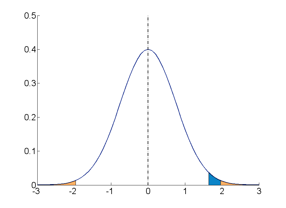
Step 4 : Your sample score of 27 needs to be converted into a Z value. To calculate Z = (27-19)/4= 2 ( check the Converting into Z scores section if you need to review how to do this process)

Step 5 : A ‘Z’ score of 2 is more extreme than the cut off Z of +1.96 (see figure above). The result is significant and, thus, the null hypothesis is rejected.

You can find more examples here:

• Statistics (RMIT Learning Lab)

Some commonly used statistical techniques

Correlation analysis, multiple regression.

• Analysis of variance

Chi-square test for independence

Correlation analysis explores the association between variables . The purpose of correlational analysis is to discover whether there is a relationship between variables, which is unlikely to occur by sampling error. The null hypothesis is that there is no relationship between the two variables. Correlation analysis provides information about:

• The direction of the relationship: positive or negative- given by the sign of the correlation coefficient.
• The strength or magnitude of the relationship between the two variables- given by the correlation coefficient, which varies from 0 (no relationship between the variables) to 1 (perfect relationship between the variables).
• Direction of the relationship.

A positive correlation indicates that high scores on one variable are associated with high scores on the other variable; low scores on one variable are associated with low scores on the second variable . For instance, in the figure below, higher scores on negative affect are associated with higher scores on perceived stress

A negative correlation indicates that high scores on one variable are associated with low scores on the other variable. The graph shows that a person who scores high on perceived stress will probably score low on mastery. The slope of the graph is downwards- as it moves to the right. In the figure below, higher scores on mastery are associated with lower scores on perceived stress.

Fig 2. Negative correlation between two variables. Adapted from Pallant, J. (2013). SPSS survival manual: A step by step guide to data analysis using IBM SPSS (5th ed.). Sydney, Melbourne, Auckland, London: Allen & Unwin

2. The strength or magnitude of the relationship

The strength of a linear relationship between two variables is measured by a statistic known as the correlation coefficient , which varies from 0 to -1, and from 0 to +1. There are several correlation coefficients; the most widely used are Pearson’s r and Spearman’s rho. The strength of the relationship is interpreted as follows:

• Small/weak: r= .10 to .29
• Medium/moderate: r= .30 to .49
• Large/strong: r= .50 to 1

It is important to note that correlation analysis does not imply causality. Correlation is used to explore the association between variables, however, it does not indicate that one variable causes the other. The correlation between two variables could be due to the fact that a third variable is affecting the two variables.

Multiple regression is an extension of correlation analysis. Multiple regression is used to explore the relationship between one dependent variable and a number of independent variables or predictors . The purpose of a multiple regression model is to predict values of a dependent variable based on the values of the independent variables or predictors. For example, a researcher may be interested in predicting students’ academic success (e.g. grades) based on a number of predictors, for example, hours spent studying, satisfaction with studies, relationships with peers and lecturers.

A multiple regression model can be conducted using statistical software (e.g. SPSS). The software will test the significance of the model (i.e. does the model significantly predicts scores on the dependent variable using the independent variables introduced in the model?), how much of the variance in the dependent variable is explained by the model, and the individual contribution of each independent variable.

Example of multiple regression model

From Dunn et al. (2014). Influence of academic self-regulation, critical thinking, and age on online graduate students' academic help-seeking.

In this model, help-seeking is the dependent variable; there are three independent variables or predictors. The coefficients show the direction (positive or negative) and magnitude of the relationship between each predictor and the dependent variable. The model was statistically significant and predicted 13.5% of the variance in help-seeking.

t-Tests are employed to compare the mean score on some continuous variable for two groups . The null hypothesis to be tested is there are no differences between the two groups (e.g. anxiety scores for males and females are not different).

If the significance value of the t-test is equal or less than .05, there is a significant difference in the mean scores on the variable of interest for each of the two groups. If the value is above .05, there is no significant difference between the groups.

t-Tests can be employed to compare the mean scores of two different groups (independent-samples t-test ) or to compare the same group of people on two different occasions ( paired-samples t-test) .

In addition to assessing whether the difference between the two groups is statistically significant, it is important to consider the effect size or magnitude of the difference between the groups. The effect size is given by partial eta squared (proportion of variance of the dependent variable that is explained by the independent variable) and Cohen’s d (difference between groups in terms of standard deviation units).

In this example, an independent samples t-test was conducted to assess whether males and females differ in their perceived anxiety levels. The significance of the test is .004. Since this value is less than .05, we can conclude that there is a statistically significant difference between males and females in their perceived anxiety levels.

Whilst t-tests compare the mean score on one variable for two groups, analysis of variance is used to test more than two groups . Following the previous example, analysis of variance would be employed to test whether there are differences in anxiety scores for students from different disciplines.

Analysis of variance compare the variance (variability in scores) between the different groups (believed to be due to the independent variable) with the variability within each group (believed to be due to chance). An F ratio is calculated; a large F ratio indicates that there is more variability between the groups (caused by the independent variable) than there is within each group (error term). A significant F test indicates that we can reject the null hypothesis; i.e. that there is no difference between the groups.

Again, effect size statistics such as Cohen’s d and eta squared are employed to assess the magnitude of the differences between groups.

In this example, we examined differences in perceived anxiety between students from different disciplines. The results of the Anova Test show that the significance level is .005. Since this value is below .05, we can conclude that there are statistically significant differences between students from different disciplines in their perceived anxiety levels.

Chi-square test for independence is used to explore the relationship between two categorical variables. Each variable can have two or more categories.

For example, a researcher can use a Chi-square test for independence to assess the relationship between study disciplines (e.g. Psychology, Business, Education,…) and help-seeking behaviour (Yes/No). The test compares the observed frequencies of cases with the values that would be expected if there was no association between the two variables of interest. A statistically significant Chi-square test indicates that the two variables are associated (e.g. Psychology students are more likely to seek help than Business students). The effect size is assessed using effect size statistics: Phi and Cramer’s V .

In this example, a Chi-square test was conducted to assess whether males and females differ in their help-seeking behaviour (Yes/No). The crosstabulation table shows the percentage of males of females who sought/didn't seek help. The table 'Chi square tests' shows the significance of the test (Pearson Chi square asymp sig: .482). Since this value is above .05, we conclude that there is no statistically significant difference between males and females in their help-seeking behaviour.

• << Previous: Probability and the normal distribution
• Next: Statistical techniques >>