how to make chapter 4 quantitative research

How To Write The Results/Findings Chapter

For quantitative studies (dissertations & theses).

By: Derek Jansen (MBA) | Expert Reviewed By: Kerryn Warren (PhD) | July 2021

So, you’ve completed your quantitative data analysis and it’s time to report on your findings. But where do you start? In this post, we’ll walk you through the results chapter (also called the findings or analysis chapter), step by step, so that you can craft this section of your dissertation or thesis with confidence. If you’re looking for information regarding the results chapter for qualitative studies, you can find that here .

Overview: Quantitative Results Chapter

• What exactly the results chapter is
• What you need to include in your chapter
• How to structure the chapter
• Tips and tricks for writing a top-notch chapter
• Free results chapter template

What exactly is the results chapter?

The results chapter (also referred to as the findings or analysis chapter) is one of the most important chapters of your dissertation or thesis because it shows the reader what you’ve found in terms of the quantitative data you’ve collected. It presents the data using a clear text narrative, supported by tables, graphs and charts. In doing so, it also highlights any potential issues (such as outliers or unusual findings) you’ve come across.

But how’s that different from the discussion chapter?

Well, in the results chapter, you only present your statistical findings. Only the numbers, so to speak – no more, no less. Contrasted to this, in the discussion chapter , you interpret your findings and link them to prior research (i.e. your literature review), as well as your research objectives and research questions . In other words, the results chapter presents and describes the data, while the discussion chapter interprets the data.

Let’s look at an example.

In your results chapter, you may have a plot that shows how respondents to a survey  responded: the numbers of respondents per category, for instance. You may also state whether this supports a hypothesis by using a p-value from a statistical test. But it is only in the discussion chapter where you will say why this is relevant or how it compares with the literature or the broader picture. So, in your results chapter, make sure that you don’t present anything other than the hard facts – this is not the place for subjectivity.

It’s worth mentioning that some universities prefer you to combine the results and discussion chapters. Even so, it is good practice to separate the results and discussion elements within the chapter, as this ensures your findings are fully described. Typically, though, the results and discussion chapters are split up in quantitative studies. If you’re unsure, chat with your research supervisor or chair to find out what their preference is.

What should you include in the results chapter?

Following your analysis, it’s likely you’ll have far more data than are necessary to include in your chapter. In all likelihood, you’ll have a mountain of SPSS or R output data, and it’s your job to decide what’s most relevant. You’ll need to cut through the noise and focus on the data that matters.

This doesn’t mean that those analyses were a waste of time – on the contrary, those analyses ensure that you have a good understanding of your dataset and how to interpret it. However, that doesn’t mean your reader or examiner needs to see the 165 histograms you created! Relevance is key.

How do I decide what’s relevant?

At this point, it can be difficult to strike a balance between what is and isn’t important. But the most important thing is to ensure your results reflect and align with the purpose of your study .  So, you need to revisit your research aims, objectives and research questions and use these as a litmus test for relevance. Make sure that you refer back to these constantly when writing up your chapter so that you stay on track.

As a general guide, your results chapter will typically include the following:

• Some demographic data about your sample
• Reliability tests (if you used measurement scales)
• Descriptive statistics
• Inferential statistics (if your research objectives and questions require these)
• Hypothesis tests (again, if your research objectives and questions require these)

We’ll discuss each of these points in more detail in the next section.

Importantly, your results chapter needs to lay the foundation for your discussion chapter . This means that, in your results chapter, you need to include all the data that you will use as the basis for your interpretation in the discussion chapter.

For example, if you plan to highlight the strong relationship between Variable X and Variable Y in your discussion chapter, you need to present the respective analysis in your results chapter – perhaps a correlation or regression analysis.

Need a helping hand?

How do I write the results chapter?

There are multiple steps involved in writing up the results chapter for your quantitative research. The exact number of steps applicable to you will vary from study to study and will depend on the nature of the research aims, objectives and research questions . However, we’ll outline the generic steps below.

Step 1 – Revisit your research questions

The first step in writing your results chapter is to revisit your research objectives and research questions . These will be (or at least, should be!) the driving force behind your results and discussion chapters, so you need to review them and then ask yourself which statistical analyses and tests (from your mountain of data) would specifically help you address these . For each research objective and research question, list the specific piece (or pieces) of analysis that address it.

At this stage, it’s also useful to think about the key points that you want to raise in your discussion chapter and note these down so that you have a clear reminder of which data points and analyses you want to highlight in the results chapter. Again, list your points and then list the specific piece of analysis that addresses each point. 

Next, you should draw up a rough outline of how you plan to structure your chapter . Which analyses and statistical tests will you present and in what order? We’ll discuss the “standard structure” in more detail later, but it’s worth mentioning now that it’s always useful to draw up a rough outline before you start writing (this advice applies to any chapter).

Step 2 – Craft an overview introduction

As with all chapters in your dissertation or thesis, you should start your quantitative results chapter by providing a brief overview of what you’ll do in the chapter and why . For example, you’d explain that you will start by presenting demographic data to understand the representativeness of the sample, before moving onto X, Y and Z.

This section shouldn’t be lengthy – a paragraph or two maximum. Also, it’s a good idea to weave the research questions into this section so that there’s a golden thread that runs through the document.

Step 3 – Present the sample demographic data

The first set of data that you’ll present is an overview of the sample demographics – in other words, the demographics of your respondents.

For example:

• What age range are they?
• How is gender distributed?
• How is ethnicity distributed?
• What areas do the participants live in?

The purpose of this is to assess how representative the sample is of the broader population. This is important for the sake of the generalisability of the results. If your sample is not representative of the population, you will not be able to generalise your findings. This is not necessarily the end of the world, but it is a limitation you’ll need to acknowledge.

Of course, to make this representativeness assessment, you’ll need to have a clear view of the demographics of the population. So, make sure that you design your survey to capture the correct demographic information that you will compare your sample to.

But what if I’m not interested in generalisability?

Well, even if your purpose is not necessarily to extrapolate your findings to the broader population, understanding your sample will allow you to interpret your findings appropriately, considering who responded. In other words, it will help you contextualise your findings . For example, if 80% of your sample was aged over 65, this may be a significant contextual factor to consider when interpreting the data. Therefore, it’s important to understand and present the demographic data.

 Step 4 – Review composite measures and the data “shape”.

Before you undertake any statistical analysis, you’ll need to do some checks to ensure that your data are suitable for the analysis methods and techniques you plan to use. If you try to analyse data that doesn’t meet the assumptions of a specific statistical technique, your results will be largely meaningless. Therefore, you may need to show that the methods and techniques you’ll use are “allowed”.

Most commonly, there are two areas you need to pay attention to:

#1: Composite measures

The first is when you have multiple scale-based measures that combine to capture one construct – this is called a composite measure .  For example, you may have four Likert scale-based measures that (should) all measure the same thing, but in different ways. In other words, in a survey, these four scales should all receive similar ratings. This is called “ internal consistency ”.

Internal consistency is not guaranteed though (especially if you developed the measures yourself), so you need to assess the reliability of each composite measure using a test. Typically, Cronbach’s Alpha is a common test used to assess internal consistency – i.e., to show that the items you’re combining are more or less saying the same thing. A high alpha score means that your measure is internally consistent. A low alpha score means you may need to consider scrapping one or more of the measures.

#2: Data shape

The second matter that you should address early on in your results chapter is data shape. In other words, you need to assess whether the data in your set are symmetrical (i.e. normally distributed) or not, as this will directly impact what type of analyses you can use. For many common inferential tests such as T-tests or ANOVAs (we’ll discuss these a bit later), your data needs to be normally distributed. If it’s not, you’ll need to adjust your strategy and use alternative tests.

To assess the shape of the data, you’ll usually assess a variety of descriptive statistics (such as the mean, median and skewness), which is what we’ll look at next.

Step 5 – Present the descriptive statistics

Now that you’ve laid the foundation by discussing the representativeness of your sample, as well as the reliability of your measures and the shape of your data, you can get started with the actual statistical analysis. The first step is to present the descriptive statistics for your variables.

For scaled data, this usually includes statistics such as:

• The mean – this is simply the mathematical average of a range of numbers.
• The median – this is the midpoint in a range of numbers when the numbers are arranged in order.
• The mode – this is the most commonly repeated number in the data set.
• Standard deviation – this metric indicates how dispersed a range of numbers is. In other words, how close all the numbers are to the mean (the average).
• Skewness – this indicates how symmetrical a range of numbers is. In other words, do they tend to cluster into a smooth bell curve shape in the middle of the graph (this is called a normal or parametric distribution), or do they lean to the left or right (this is called a non-normal or non-parametric distribution).
• Kurtosis – this metric indicates whether the data are heavily or lightly-tailed, relative to the normal distribution. In other words, how peaked or flat the distribution is.

A large table that indicates all the above for multiple variables can be a very effective way to present your data economically. You can also use colour coding to help make the data more easily digestible.

For categorical data, where you show the percentage of people who chose or fit into a category, for instance, you can either just plain describe the percentages or numbers of people who responded to something or use graphs and charts (such as bar graphs and pie charts) to present your data in this section of the chapter.

When using figures, make sure that you label them simply and clearly , so that your reader can easily understand them. There’s nothing more frustrating than a graph that’s missing axis labels! Keep in mind that although you’ll be presenting charts and graphs, your text content needs to present a clear narrative that can stand on its own. In other words, don’t rely purely on your figures and tables to convey your key points: highlight the crucial trends and values in the text. Figures and tables should complement the writing, not carry it .

Depending on your research aims, objectives and research questions, you may stop your analysis at this point (i.e. descriptive statistics). However, if your study requires inferential statistics, then it’s time to deep dive into those .

Step 6 – Present the inferential statistics

Inferential statistics are used to make generalisations about a population , whereas descriptive statistics focus purely on the sample . Inferential statistical techniques, broadly speaking, can be broken down into two groups .

First, there are those that compare measurements between groups , such as t-tests (which measure differences between two groups) and ANOVAs (which measure differences between multiple groups). Second, there are techniques that assess the relationships between variables , such as correlation analysis and regression analysis. Within each of these, some tests can be used for normally distributed (parametric) data and some tests are designed specifically for use on non-parametric data.

There are a seemingly endless number of tests that you can use to crunch your data, so it’s easy to run down a rabbit hole and end up with piles of test data. Ultimately, the most important thing is to make sure that you adopt the tests and techniques that allow you to achieve your research objectives and answer your research questions .

In this section of the results chapter, you should try to make use of figures and visual components as effectively as possible. For example, if you present a correlation table, use colour coding to highlight the significance of the correlation values, or scatterplots to visually demonstrate what the trend is. The easier you make it for your reader to digest your findings, the more effectively you’ll be able to make your arguments in the next chapter.

Step 7 – Test your hypotheses

If your study requires it, the next stage is hypothesis testing. A hypothesis is a statement , often indicating a difference between groups or relationship between variables, that can be supported or rejected by a statistical test. However, not all studies will involve hypotheses (again, it depends on the research objectives), so don’t feel like you “must” present and test hypotheses just because you’re undertaking quantitative research.

The basic process for hypothesis testing is as follows:

• Specify your null hypothesis (for example, “The chemical psilocybin has no effect on time perception).
• Specify your alternative hypothesis (e.g., “The chemical psilocybin has an effect on time perception)
• Set your significance level (this is usually 0.05)
• Calculate your statistics and find your p-value (e.g., p=0.01)
• Draw your conclusions (e.g., “The chemical psilocybin does have an effect on time perception”)

Finally, if the aim of your study is to develop and test a conceptual framework , this is the time to present it, following the testing of your hypotheses. While you don’t need to develop or discuss these findings further in the results chapter, indicating whether the tests (and their p-values) support or reject the hypotheses is crucial.

Step 8 – Provide a chapter summary

To wrap up your results chapter and transition to the discussion chapter, you should provide a brief summary of the key findings . “Brief” is the keyword here – much like the chapter introduction, this shouldn’t be lengthy – a paragraph or two maximum. Highlight the findings most relevant to your research objectives and research questions, and wrap it up.

Some final thoughts, tips and tricks

Now that you’ve got the essentials down, here are a few tips and tricks to make your quantitative results chapter shine:

• When writing your results chapter, report your findings in the past tense . You’re talking about what you’ve found in your data, not what you are currently looking for or trying to find.
• Structure your results chapter systematically and sequentially . If you had two experiments where findings from the one generated inputs into the other, report on them in order.
• Make your own tables and graphs rather than copying and pasting them from statistical analysis programmes like SPSS. Check out the DataIsBeautiful reddit for some inspiration.
• Once you’re done writing, review your work to make sure that you have provided enough information to answer your research questions , but also that you didn’t include superfluous information.

If you’ve got any questions about writing up the quantitative results chapter, please leave a comment below. If you’d like 1-on-1 assistance with your quantitative analysis and discussion, check out our hands-on coaching service , or book a free consultation with a friendly coach.

Psst... there’s more!

This post was based on one of our popular Research Bootcamps . If you're working on a research project, you'll definitely want to check this out ...

You Might Also Like:

Thank you. I will try my best to write my results.

Awesome content 👏🏾

this was great explaination

Submit a Comment Cancel reply

Your email address will not be published. Required fields are marked *

Save my name, email, and website in this browser for the next time I comment.

• Print Friendly

• Chapter Four: Quantitative Methods (Part 2 - Doing Your Study)

Now that you have designed your study, you can commence with collecting and analyzing your data, which is the topic of this section of the chapter. Some professors will want you to actually present a proposal of your study to them before you begin collecting data, and you will need to get IRB approval for starting your data if you are going to ever be using this data for a paper or presentation outside of class. Check with your professor before collecting data to see if these two steps are necessary for the project for their class.

• Chapter One: Introduction
• Chapter Two: Understanding the distinctions among research methods
• Chapter Three: Ethical research, writing, and creative work
• Chapter Four: Quantitative Methods (Part 1)
• Chapter Four: Quantitative Methods (Part 3 - Making Sense of Your Study)
• Chapter Five: Qualitative Methods (Part 1)
• Chapter Five: Qualitative Data (Part 2)
• Chapter Six: Critical / Rhetorical Methods (Part 1)
• Chapter Six: Critical / Rhetorical Methods (Part 2)
• Chapter Seven: Presenting Your Results

Data Collection

Contacting participants.

Where are you going to find your participants? Is the population from which you can draw your participants in a list that you can access somewhere? If so, then you may be able to do some sort of probability or random sample, as discussed in the previous section of this chapter. In that case, getting the people who "own" the list to give you permission to use the list will be your major challenge. Sometimes they might want you to let them do the random sample and send out the invitation to participate, as the list is private.

At other times, and probably most commonly for communication researchers, there is no set population list from which you can draw a random sample. Then you have to decide what participants might be likely to agree to participate in your study. Is there a certain characteristic they have to meet (e.g., if you are doing a study of online dating, do they have to have participated in online dating) in order to be in your study? If so, then you need to "go" places where those people might be gathering, such as online chat rooms or Facebook groups specifically focusing on online dating.

If there are no specific characteristics of your population, but you just want a certain number of males and females, for example, or you want to gather college students' perceptions, then you will go with a  convenience sample , and contact people however you can. You can rely on people you know through Facebook, go to classes and ask for participants, select people you see in the union, etc. You may also rely on your participants to spread the word about your study to people they know, thus collecting a  snowball  or  network sample .

The main thing you need to remember as you are contacting possible participants, besides following the human participants procedures you learned about in chapter three and that you promised to do in your Institutional Review Board (IRB) application, is to keep track of the methods you are using while contacting them, as you will have to report what you did in the methods section of your eventual paper or report.

Getting Informed Consent

Most of the time, university institutional review boards (IRBs) require you to get "informed consent" from the participants before they complete a survey or participate in your study. This process was discussed in chapter three. Sample informed consent form templates can be found at your university's website (e.g.,  IRB Forms ).

Even if you are in a workplace, gathering data after you graduate, and are not required to get IRB permission to do your study, it is still a good idea to provide the opportunity for your participants to give "informed consent" before beginning your study. This will help protect you legally if there was a question about your study afterwards.

For online surveys (such as those on surveygizmo.com and surveymonkey.com), you often can build in your informed consent within the first page of the survey, so that if they continue taking the survey, they are consenting to the survey conditions and risks/benefits. An example of language April has used on such an online survey is included below, along with her recruiting script used when she directed people to the online survey.

Example recruiting script.

Seven years ago, my husband and I adopted our first precious daughter from China (who is now 8 years old). We went back 2 1⁄2 years later for our second daughter (who is now 6 years old). We recently returned from a return trip to China where we visited both of our daughters' orphanage cities. Since returning, I have become interested as part of my work as an Associate Professor in the Dept. of Communication Studies at the University of Northern Iowa, on why people take such trips and the impact of these trips on adoptive families. If you would be interested in participating in a 10-15 minute online anonymous survey on this topic, please go to the link below.

Nature and Effects of Return Trips to China for Adoptive Families

If you would like more information on the study, feel free to e-mail me at  [email protected] .

Dr. April Chatham-Carpenter

Example online informed consent

Seven years ago, my husband and I adopted our first precious daughter from China (who is now 8 years old). We went back 2 1⁄2 years later for our second daughter (who is now 6 years old). We recently returned from a return trip to China where we visited both of our daughters' orphanage cities. As part of my responsibilities as an Associate Professor at the University of Northern Iowa, I had the opportunity while in China to present a paper, at an international intercultural communication conference in Beijing, on how we as adoptive parents talk to our children about their adoptions and about their homeland.

I am now doing a two-part study, the first of which is a survey of adoptive parents who have participated in a return trip to China with their adoptive child/ren. I am interested in finding out the nature of such trips, as well as what perceived effects such trips have on adoptive families.

Although you will receive no direct benefits from participation in the study, the results obtained may offer a better understanding of return trips to China for adoptive families. There is no way to identify you from the survey, as your answers will be completely anonymous, unless you indicate on the last question of the survey that you would be interested in participating at a later time in Part Two of the study, which is an in-depth interview about your trip/s. If so, I would change all of the names and identifying information in any report that is written/presented, so that you would not be able to be identified.

Besides the approximate 10-15 minutes it would take you to complete the survey, there are no perceived risks from participating in this study. If, however, at any time you become uncomfortable answering the survey questions, you may discontinue your participation in my study, or you may submit only selected answers to the questions. Your participation is voluntary.

If you have any questions about this research or about your rights as a research participant, you may feel free to contact me directly, Dr. April Chatham-Carpenter, at 319-273-5901, or my university's Institutional Review Board Office at 319-273-6148.

Thanks for taking the time to fill out the survey below. Completion and submission of the survey implies that you have read the information above and consent to take part in the research. Make sure to hit the "submit" button at the bottom of the survey when you have answered the questions you'd like to answer. A few of the questions, marked by a red star, are required for the survey to be submitted.

It is sometimes difficult to get informed consent if you are observing unobtrusively in a setting. Then you have to rely on your own ethical judgment as to whether you are potentially harming the people you are observing by your observations. One good question to ask is "how would I feel if someone was watching me in this way and not telling me"? If you would answer, "I would not want them to do this," then that should be a red-flag for you to not do your observations without asking for permission to do so from your participants.

Collecting Data

After you have recruited participants to participate, you begin collecting data. How active you are in this process depends on what type of data you are collecting. If you are collecting face-to- face data of some kind, then you will be very busy collecting data.

If you are collecting online data, then you wait and see how many people respond to your online survey. It is helpful for this type of data collection to send out a couple of reminder announcements about a week apart before closing the survey. If you are not getting the kind of response at that point that you wanted, then you might consider attempting to find possible participants in additional ways. April had a graduate student one semester who had to contact various businesses for permission to send her recruitment script to their employees, as well as using several university graduate student listservs, before she reached her goal of having 100 people respond. (Remember, even if you do not have a random sample, the larger your sample, the better you will generally be able to generalize to your population.)

After you have met your goal of the size of sample you wanted, then you can go next to analyzing your data, which is covered in the next section.

Data Analysis

Context for use of statistics: accounting for data.

When you collect data for a research study, you have to tell a "story" about the data you collected. This "story" uses your data to provide the answer to your research question/s or hypothesis/es. For quantitative studies, you rely on "counts" or numbers to support the story you are telling. These counts are made up of summary data, sometimes called "descriptive statistics" as seen in the next section, as well as statistical tests, often called "inferential statistics" as seen below. These statistics are just numbers that help us answer our research question/s or test our hypothesis/es. Remember when we talked about sampling earlier, we said that statistics are estimates of population "parameters," and since we cannot measure the whole population, we rely on statistics instead of population parameters such as those used in a census, for example.

If you are feeling scared already, no need to be. We will be using SPSS (Statistical Package for the Social Sciences) to compute the statistics. SPSS provides already developed computer programs to run the statistical tests. You will most likely not have to be computing any statistics by hand, except perhaps to learn how the statistic works. Your job will be to input the data and tell SPSS which type of statistical tests to run. In general, the form of research question or hypothesis you pose will dictate the type of statistics needed.

Putting Data into SPSS

If you do not want to compute your statistics by hand, the first thing you will need to do is to enter your data into SPSS or some other statistical package software. We suggest SPSS because all of the computer labs on campus have this package readily available.

There are many good free resources that explain how to use SPSS, as well as YouTube videos you can watch. We have listed a few here, so you can go to them to help you enter your data, "clean" your data, and run the necessary statistics to answer your research question/s or test your hypothesis/es. We also provide some basic statistical procedures using SPSS for the statistical tests we will explain.

Website Links

SPSS On-Line Training Workshop

YouTube Videos

Type in "SPSS tutorial" into YouTube, and you will find helpful videos such as the following. As we get further along to looking at specific types of statistics, you can also type in the name of the test and SPSS into the search box, and it will provide you a tutorial.

Intro to SPSS SPSS 1 Quickstart: Extracting Data

Surveygizmo » SPSS

One tutorial that is helpful for students is how to take survey results from an online survey (in this case we use surveygizmo.com to illustrate because that is April's favorite online survey source) and transfer the data into SPSS. We provide that below in three steps. To get a surveygizmo account, go to the following website to get one: Online Survey Tool for Students .  These accounts sometimes allow you to export your data directly into SPSS. If so, then you can disregard the following tutorial.

To run your report, click on Reporting » Reports » Summary [under "create a new report"]. Indicate you want to "just display multiple choice questions" [so open-ended questions are not included for the sake of SPSS]. Then click on "create report," and then click on "report runs" on the left hand side, and click on the "run report now" button, when it appears. At that point, it will run your report, and that report will show up under "your saved reports" when you click on reporting » reports in the future. To access the results, you then click on the report name under the "your saved reports" area, and it will give you the results in table form, representing the descriptive statistics.

• Delete unneeded, non-data columns. (right-click on top of column – A-Z symbol)
• Delete unneeded, non-data row/s. (right-click on row #)
• Except for open-ended questions, for non-numeric data, you will need to convert the words to #s, if not already done. Do this column by column, right-clicking on the capital letter above the column and then using "find & select » replace" option. Write down what the numbers mean on a blank survey – you will need them later for your SPSS file labels. For any "check all that apply" questions, make the filled in column be "1". If they didn't check that option, it will be left blank.
• Save file!!!  
• Open up SPSS » type in data
• Cut & paste each column you want copied into SPSS, using Data View button on lower left-hand of screen. (You can do all columns all at once, as long as they have been converted to numbers.)
• Create variable names, labels, and values, as needed in the file for the #s you created in "clean up" step 1 above, from Variable View button on lower left-hand side of screen.
• Save file often!!!

Descriptive Statistics

After you have your data in an SPSS data file, you can start running your statistics. The first kind of statistics you will want to run are "descriptive" statistics. Descriptive statistics fall into two major types: "central tendency measures" and "variability measures." Together they provide an overview or a general picture of your data. We will also discuss other types of descriptive statistics, i.e., the frequency and percentage. All of these types of statistics are the easiest ones to compute by hand, as will be seen below.

Central Tendency Measures

Central tendency measures are statistics which tell you what the "average" score on a particular survey item or measure is. They consist of three types: mean, median and mode.

The  mean  is the one we are most used to, in everyday life. It is the arithmetic average of a data set, where you add up all of the scores and divide them by the total number of participants. Means are used for continuous level data (i.e., ordinal, interval, and ratio data). What is the mean of the dataset below? (Did you also get a mean of 5?)

1, 1, 2, 2, 2, 3, 4, 4, 4, 4, 5, 5, 6, 7, 7, 7, 8, 9, 9, 10

When you have nominal/categorical data, then you need to use the  mode , which is the most frequent score or answer. It is often called the "modal" answer. You can also determine the mode of continuous level data, such as the dataset above. What is the mode for the above dataset? (Note: You can have multiple modes, but in this case you do not, as 4 is the most frequent answer.)

Ordinal data can use all three types of averages, but commonly uses the  median , which is the point/score at which 50% of the cases fall above and 50% fall below (e.g., median home price). You can also figure out the median for the above dataset, which would be between the numbers 4 and 5, thus 4.5.

Variability Measures

Variability measures deal with how much difference or variability there is between scores in the same dataset. For example, imagine you are a teacher, you gave the same test in two different classes and now you want to see how the classes compared. You may find in one class there was a great deal of variability between individual scores (cf. Chart 2 below), while in the other you may find scores group closely together around the mean (cf. Chart 1 below). There are three measures of variability used by researchers: range, variance, and standard deviation.

The  range  is the difference between the highest and lowest score in a data set. For the given dataset we have been working with (pasted below for your convenience also), what is the range?

Did you say a range of 9 (the lowest number, 1, subtracted from the highest number, 10)?

The  variance  is how much difference there is between scores, or the average of the squared deviations around the mean. Let us work with this same dataset to compute the variance. The mean of the dataset above, as we determined earlier, is 5.

Now we have to compare each number to the mean of the dataset.

Then you square all of these numbers, as seen in parentheses above; add up the squared deviations from the mean (= 146 here); and compute the average squared deviation from the mean, i.e., the variance (by dividing by the total number of scores, which is 20 here). The variance for this data set is 7.3.

The third measure of variability is the  standard deviation , which is the square root of the variance (in this case, it is 2.70). When researchers report means, they will almost always report the standard deviation scores, because this provides readers an indication of how much variation in the sample there is. In Chart 1 below, there is very little variation among the sample, but in Chart 2, there is quite a bit of variation. The standard deviation statistic provides you information on this. If the standard deviation is large, then it will look like Chart 2, but if it is small, it will look more like Chart 1.

To see an example of a table used in an actual research study which uses both means and standard deviations, check out Table 1 (p. 516) from the following article.

In this article, the authors reported the means and standard deviations for personality characteristics displayed by three different roles the fictional President Bartlett played on the show.

Frequencies & Percentages

Other descriptive statistics also commonly reported include frequencies and percentages of answers given to survey questions. For example, the Association of American Colleges and Universities (2010) contracted a research group to interview 302 employers in 2009 about their views on college learning in the midst of the economic decline. Throughout this article (which can be found here:  Employer Survey ), they report the percentage of employers who state certain expectations of college graduates. One finding communication students might find interesting is that 89% of the employers believed schools should put an emphasis on "the ability to communicate effectively, orally and in writing" (p. 2). One finding your textbook authors were grateful for, in light of the topic of this course, was that 81% of employers said that it would help "a lot" or a "fair amount" for "students [to] develop the skills to research questions in their field and develop evidence-based analyses" (p. 8).

Sometimes it is helpful to compute a frequency distribution to be able to better visualize the results of a study. For example, for the dataset we used earlier, here is what the frequency distribution would look like.

If you decided you wanted to represent the data using another type of chart, e.g., a bar graph, the data might look like this.

For more information on what other things you can do with frequency distributions, along with how to create them using SPSS, check out the following website: Frequency Distribution

Running the Statistics

All of the statistics we have run so far can be computed by hand, but many students prefer (especially if they have a large number of participants) having the computer do this work for them. Once you have converted your data into SPSS, then running the needed statistics is very easy.

You can get all of the statistics we have talked about so far in SPSS from the "analyze" tab at the top of the SPSS interface screen and click on, in order: analyze » escriptive statistics » frequencies » statistics (choose which ones you want). Then enter the variables you want to have entered.

Inferential Statistics

Descriptive statistics merely describe a sample and cannot be used to make any conclusions beyond your participants. When you wish to "infer" or generalize beyond your sample to a larger population on your findings, you have to use what are called "inferential" statistics.

Background on Inferential Statistics

Inferential statistics always generate probability or p-levels. In part 2 of this chapter, we discussed how p-levels represent statistical "significance," or the probability of finding a "significant" answer only by chance, when no such relationship between variables actually exists in a particular subject population. When you read in an article that a finding was significant at the commonly accepted "p< .05" level, it means that if you ran the study 100 times, you would obtain this observed difference by chance only 5 times, so you can be 95% confident that you would find this same finding in the actual population as well. These probability levels allow you to generalize to a larger population.

For more information on probability levels in terms of hypothesis testing, see the following YouTube video: p Value Explained .

For more examples explaining the concept of probability in general, see the following website: Certain and Impossible Events .

As noted in Part 1 of this chapter, in quantitative research, you will often hear people talk about "null" and "alternative" hypotheses. The "null" hypothesis is that there is no significant difference or association between the variables you are studying, and the "alternative" hypothesis is that there is a significant difference or association between the variables you are studying. If you reject the null hypothesis and accept the alternative hypothesis, then that means your inferential statistics are showing statistically significant results at p<.05.

For more information on null and alternative hypotheses, see the following websites. Hypothesis Testing Hypotheses

The researcher might, however, make a wrong decision when using p-values. Researchers talk about these wrong decisions as Type I and Type II errors, as we earlier mentioned when discussing sampling. A Type I error is the same as our p-value, and is the likelihood that we have rejected the null hypothesis when we should not have. A Type II error is the likelihood that we have accepted the null hypothesis when we should not have.

In addition to the websites referenced when talking about sampling, more explanation on these types of errors can be found at the following website:  Type I and Type II Errors - Making Mistakes in the Justice System .

There are many types of inferential statistics. We will talk about two overall types of tests: (a) tests of difference (used with difference research questions or hypotheses), and (b) tests of association/relationship (used with association/relationship research questions or hypotheses). Tests of difference answer questions such as, "is there a  difference  between first-year and fourth- year students on their use of facebook," while tests of association/relationship answer questions such as, "is there a  relationship  between first-year students' GPAs and the time it takes them to graduate" and "what are the best predictors of time to graduation."

Tests of Difference

Tests of difference ask the question, "are the  differences  observed between the categories of the independent variable (IV) with respect to the dependent variable (DV) due to chance or are they real differences in the population?" Because tests of difference are always used with research questions or hypotheses of difference, looking at differences between groups (see Part 1 of this chapter for a review of what these kind of questions/hypotheses look like), the independent variable is always categorical in nature, meaning it is nominal (and sometimes ordinal), and the dependent variable is always continuous (interval or ratio).

Which difference test you run depends on the number of independent variables you have and how many levels there are for your independent variable (if you only have one). See the chart below to help you choose the most appropriate difference test for your difference research question/hypothesis.

The first test of difference we discuss in this section is the  t-test . T-tests are used to test the significance of differences between the means of TWO groups or populations on some dependent variable. For example, in April's home schooling study, she wanted to know if there was a significant difference between home and public schooled adolescents on the total number of contacts each group had over a month's period of time. The home schoolers in her study had an average of 49.29 distinct contacts, and the public schoolers had 56.25. Was that difference a statistically significant one? The actual t-test results she found could have been written as follows

A t-test with the unequal variances solution showed the difference in number of contacts for home (m = 49.29) and public (m = 56.25) schooled participants to not be a significant one, t (38.8) = -0.6319, p = .5312.

Suppose, however, she had found a significant difference, with different means per group. She might then have written:

A t-test with the unequal variances solution showed the difference in number of contacts for home (m = 35) and public (m = 60) schooled participants to be significant, t (38.8) = 2.4317, p = .001.

There are two overall types of t-tests: (a) the t-test for independent samples, and (b) the paired samples t-test. The basic difference between these two tests is whether the two groups being compared are related in some way. For example, if you are doing a pretest and posttest on the same subjects, and they are measured more than once, the two scores being compared are related, and you would use the paired samples t-test. If you were collecting relationship satisfaction scores from both partners in a relationship, and you were comparing them to see if they were different from each other, then you would use the paired samples t-test. But, however, if you were interested in whether young-married couples and older-married couples differed in their relationship satisfaction, then you do not have groups that are related in any way, and you would use the t-test for independent samples.

Both types of t-tests are very easy to run using SPSS. View the YouTube tutorials below to find out how.

Running a T test in SPSS  (independent samples t- test) 2.3 Paired Samples T Test: PASW (SPSS) Statistics v.17 video  (paired-samples t-test)

Analysis of Variance (ANOVA)

A researcher chooses to use ANOVA when s/he has is testing for the significance of differences between means among groups/populations with one of the following conditions: (a) a single categorical/nominal IV with THREE or more levels (e.g., home vs. public vs. private schooling), or (2) two or more categorical IVs (e.g., type of schooling & biological sex).

The reason these tests are called analysis of variance is because there are two possible sources of variability in a sample's scores on a test like self-esteem, for example. There are differences  between  the groups being compared, and that is called "between-groups variance," and there are differences  within  each group, and that is called "within-groups variance" (sometimes also called "error" or differences within the groups occurring just by chance). The formulas for computing ANOVA look closely at both of these types of variance, thus the test is called analysis of variance.

If you are interested in reading more about the formula for ANOVA tests and how it is related to the study of these two different types of variance, take a look at one of the following websites.

Psych. Statistics: One way analysis of variance (ANOVA) One-way ANOVA

One-way ANOVA

The first type of ANOVA is called a one-way ANOVA. It has one categorical independent variable, with more than two levels, and one continuous dependent variable. An example from the world of psychology can be found at the following website:  Between Subjects One-Way ANOVA example , in a study that explored learning differences between students exposed to different types of background sound.

One-way ANOVA is also used by communication scholars, as illustrated by the following article, who did a content analysis of children's television programming.

McCollum Jr., J. F. & Bryant, J. (2003). Pacing in children's television programming.  Mass Communication and Society, 6  (2), 115-136.

One of their hypotheses was the following: "There will be significant differences in individual pacing criteria among networks, with the commercial networks having the faster pace" (p. 118). They compared pacing between several different networks (more than two), thus they needed to use ANOVA. One of the ways the authors of this article measured "pacing" was through how often camera cuts or edits were done between characters on the show. They used a one-way ANOVA to test their hypothesis, concluding:

An analysis of variance (ANOVA) on the frequency of camera edits yielded a statistically significant main effect for network, with F(4, 80) = 4.21, p = .004. The programs on PBS ( M  = 38.27) and The Learning Channel ( M  = 38.20) had a statistically significantly smaller number of camera edits per segment than did the programs on the commercial networks ( M  = 59.87) and the Disney Channel ( M  = 64.27). Nickelodeon ( M  = 51.47) fell between and did not differ significantly from any other channel in frequency of camera edits. (McCollum & Bryant, 2003, pp. 129-130)

To understand how you can use SPSS to run the one-way ANOVA test, see the following two sources:

ANOVA with SPSS  (this source covers all kinds of ANOVA testing) and  SPSS: ANOVA (2 in 1) .

Two-way and factorial ANOVAs

A two-way ANOVA has two independent categorical variables and one continuous dependent variable. Two-way and above ANOVAs are also called factorial ANOVAs, because they have multiple "factors" or independent variables. You technically could have three-way (with three independent variables), four-way (with four independent variables), etc. ANOVAs, but it is easier to call anything above a two-way ANOVA a factorial ANOVA.

Sometimes researchers write up their methods with a description of these types of designs by indicating how many levels each of their independent variables have. A researcher who has a 2 (biological sex) X 3 (type of schooling) X 4 (classification level) ANOVA would have three independent variables, and the numbers between the X's indicate how many levels each of the independent variables have.

Paul Witt and Paul Schrodt (2006) did a study of 549 college students and their perceptions of their instructor based on levels of technology use and teacher immediacy behaviors. They had a 4 (four levels of technology use: non, minimal, moderate, complete) X 2 (immediacy: highly immediate & nonimmediate) factorial ANOVA.

Witt, P. L., & Schrodt, P. (2006). The influence of instructional technology use and teacher immediacy on student affect for teacher and course.  Communication Reports, 19 (1), 1-15.

To understand how you can use SPSS to run these types of ANOVAs, see one of the following websites.

Factorial Design (Part B): Data Analysis with SPSS Two-Way ANOVA - SPSS for Homework ANOVA with SPSS

There are several tests which will be run in a factorial ANOVA to test for significance. These tests are divided into "main effects" and "interaction effects." In April's home schooling study, imagine that she was interested to see if there were differences in not only home vs. public schooled adolescents, but also between young, middle, and older adolescents, in the total number of contacts they had over a month's period of time. She would then have a 2 (type of schooling) X 3 (age group) ANOVA design with this test.

In this example, April might actually have had three separate research questions: (a) is there a difference between home and public schooled adolescents in the total number of contacts they communicated with over a month's period of time; (b) is there a difference between young, middle, and older adolescents in the total number of contacts they communicated with over a month's period of time; and (c) is there an interaction between age and schooling type on total number of contacts. The first two research questions would test for what is called "main effects" or "between-subjects effects." Both type of schooling and age served as her "main effects," and a factorial ANOVA would test for differences between the means of the groups for each of the main effects, as seen in the table below.

In this case, both the main effects would probably be significant, as their means look quite a bit different. To test where the difference was between the age groups, however, April would have to do what are called "post hoc tests," which are tests you do after you find out you have a significant difference between three or more groups and you want to find out which groups are significantly different from each other. There are many different types of these post hoc tests, and thankfully SPSS will conduct them for you, if you ask it to do so in the "post hoc" dialogue box provided for either the one-way ANOVA or factorial ANOVA.

It is beyond the scope of this course text to talk about these different types of post hoc tests, but April likes the Tukey test personally.

See also the following website if you would like more information on doing such a test with SPSS:  One-way ANOVA .

By doing a factorial ANOVA, April would also have wondered if schooling type and age interacted in some way, such as might be seen in the following graph, thus answering the third research question above. If the lines cross and/or are not parallel, as seen here, it means there is likely to be a significant interaction between these two variables.

Witt and Schrodt (2006), in the study mentioned earlier, found significant main effects for both technology use and teacher immediacy, as well as a significant interaction effect between those two independent variables.

If you would like more information on main and interaction effects, see the following websites.

Factorial Between-Subjects ANOVA What is an Interaction?

For information on how to write up factorial ANOVA results, see the following websites. The first one shows how to do the SPSS analysis for the write-up, and the second one shows how to write up the results.

Project 2Way ANOVA - SPSS Writing Up Two-Way ANOVA

The third difference test we discuss in this section is the chi-square test. As seen in the decision flow-chart in this section of the chapter, the chi-square test is used with categorical (usually nominal) variables only. It specifically is used to test whether the actual  frequency  of occurrence of responses in a particular set of categories differs from what might be expected or what might occur by chance. It uses frequency data rather than means, since you are dealing with nominal or categorical data.

Often a researcher chooses to perform a chi-square test when s/he has content analysis data, because that data usually involves frequency counts. For example, Counsineau, Rancourt, and Green (2006) used a chi-square to test the results of their content analysis of online message boards dealing with menopause, to see if what they found was significant.

Cousineau, T. M., Rancourt, D., and Green, T. C. (2006). Web chatter before and after the women's health initiative results: A content analysis of on-line menopause message boards.  Journal of Health Communication, 11 (2), 133-147.

Goodness of fit chi-square

There are two different types of chi-square analyses you can do. The first one is the "goodness of fit" chi-square in which you only have one variable you are testing for significance, i.e., only one group of frequencies. For example, if Victoria and April had decided to do a content analysis on their qualitative self-esteem data, they could have coded one or more of their open-ended questions into inductively-derived categories 1 , and determined how often each theme or category was used. The "goodness of fit" chi-square would allow them to see if the frequencies for each theme were significantly different than what would be expected by chance. It tests to see if the expected frequencies (usually the same number per category) are the same as the observed frequencies.

If, for example, there were 5 categories developed from the data as to how the women in the study enhance their self-esteem, the chi-square goodness of fit test would expect there to be an equal number of choices of each category among the women. However, if each category was not chosen equally, there would be a difference between the observed and expected frequencies, and the chi-square would find this difference as significant.

Pearson et al. (2007) asked the following research questions in a study of how speech anxiety was covered in public speaking textbooks: "Are there overall differences in the total length of coverage used by each of the public speaking textbook authors to discuss CA?" and "Are there overall differences in the total length of coverage for each CA topic in the top ten public speaking textbooks?" (p. 161) They tested the data they coded for statistical significance using a "goodness of fit" chi-square (or what they called a "one sample" chi-square). To read about their results, check out their article.

Pearson, J. C., DeWitt, L., Child, J. T., Kahl Jr., D. H., and Dandamudi, V. (2007). Facing the fear: An analysis of speech-anxiety content in public-speaking textbooks. Communication Research Reports, 24(2), 159-168

To see how you might do a goodness of fit chi-square using SPSS, watch the following YouTube tutorial:  SPSS Chi-Square Goodness-of-Fit .

Test of independence

The second type of chi-square test is the test of independence, and involves a categorical independent variable and a categorical dependent variable. This differs from the ANOVA and t-test procedures because the dependent variable is not continuous in nature, as is required by the ANOVA and t-test statistics.

An example of the test of independence chi-square is illustrated at the following website, where their independent variable was biological sex and their dependent variable was whether a person died or survived on the Titanic, with both variables being categorical in nature. Chi-Square in SPSS

Medved et al. (2006) coded over 900 messages collected about parental work and family balance into 21 categories, and found, using chi-square, that men and women reported receiving similar messages about work and family, although there were some differences on who received "stopping work" after children messages, with women receiving more of these than men, after having children. They tested their data with a chi-square "test of independence," since their independent variable, biological sex, and their dependent variable, the categories of messages, were both nominal in nature. If you would like to read more about this study, check it out with the full citation below.

Medved, C. E., Brogan, S. M., McClanahan, A. M., Morris, J. F., & Shepherd, G. J. (2006). Family and work socializing communication: Messages, gender, and ideological implications.  Journal of Family Communication, 6 (3), 161-180.

To understand how to do a test of independence chi-square test using SPSS, go to the following YouTube tutorial:  Chi-Square analysis on SPSS .

Tests of Association or Relationship

Tests of association or relationship do not look for differences between groups, as the tests of difference do. Rather, they are used with research questions/hypotheses of association/relationship. You use these types of tests when you are exploring or testing the relationship between two or more variables. Typically, the variables used in these types of tests are all continuous in nature. We will look at two of these types of tests: (a) correlation and (b) regression. Often the independent variables are called "predictor" variables in these types of tests, and the dependent variables are called "criterion" or "outcome" variables.

Correlation

When you want to see if two or more variables covary or change with each other, then you are looking for a relationship between these variables. For example, when April noticed that there was a wide range of number of contacts for the home schoolers she studied, she wondered if age was related to the number of contacts, or if size of church youth group (since all of her home schoolers were religiously affiliated) was related to number of contacts they had. In order to find this out, she would have to conduct multiple correlation tests.

For each correlation done, for each person or group, their independent and dependent variable scores are matched. In the case of April's study, a person's age (IV) and number of contacts (DV) was matched, and the size of a person's youth group (IV) and number of contacts was matched. Often researchers will plot these matches on what is called a "scatterplot," to be able to visually see if there is a relationship between the two variables (see below, from  netmba.com ). The closer the dots plotted are to a line that can be drawn through the data, the greater the relationship or correlation is between the two variables.

The measure for a test of relationship/association for interval/ratio variables is Pearson's r (Pearson's product-moment correlation) 2 , and it can range from a "-1" to "+1." The  size  of the number (correlation coefficient) indicates how large or small the relationship is, and the  sign  indicates the direction of the relationship (positive or negative).

If the relationship between the variables is positive, as the value of one variable (e.g., age) goes up, then the value of the other variable (e.g., number of contacts) goes up. If it is negative, that means that as the value of one variable goes up (e.g., self-esteem), the value of the other variable goes down (e.g., communication apprehension).

To see how a variety of values might create different visual scatterplots, including positive and negative correlations, input some numbers into the following website:  Scatter Plot and Line of Best Fit .

In April's home schooling study, she indeed did find there was a positive correlation between church youth group size and total social network size for her participants. (She did not actually test the relationship between age and social network size.) She stated the following:

Overall, there was a positive correlation between church youth group size and total social network size,  r  (39) = .33533,  p  < .0321, meaning that as church youth group size increased so did the number of contacts a participant reported. This correlation was larger for the home schooled participants,  r  (19) = .45996 ( p  < .0359), than for the public schooled participants,  r  (18) = .21743 ( p  < .3571). (Chatham, 1991, p. 194)

How large the relationship is (i.e., as the correlation coefficient, r, gets closer to 1 or -1) helps explain how much predictive power one variable has for another variable. This predictive power is specifically measured by squaring the r value to get "R-squared" or the "coefficient of determination." In April's study, the coefficient of determination for the home schoolers was 0.21156 (the square of .45996). This value tells the researcher how much of the variance of one variable is accounted for by the other variable.

In April's study, the R-squared value of 0.21156 means that 21% of the variability in the social network size among all of her home schoolers (it ranged between 7 to 150 contacts over a month's period of time, so there was a lot of variability among her participants) can be accounted for or explained by the size of the church youth group. There are, however, still a lot of other possible predictors which can help explain a home schooler's social network size; 79% of the variance between the home schoolers was not explained by the size of the church youth group.

See the following YouTube video to better understand the coefficient of determination:  Coefficient of determination (r-squared) .

Even though we can use the coefficient of determination or R-squared to account for variance in one variable by the other variable, we cannot prove causation by correlational data. We do not know, for example, in April's study, if the home schoolers went to a larger church and therefore had a larger social network, or if perhaps they had more social contacts and therefore wanted to go to a larger church.

For more information on the difference between correlation claims and causation claims, see the following source:  Correlation does not imply causation .

To learn to compute correlation statistics on SPSS, check out the following YouTube tutorial:  Correlation Coefficients in SPSS/PASW .

If you wish to go further than correlation and actually try to predict a person's score on a dependent variable by knowing their score on an independent variable, you should use regression. Regression attempts to find the "line of best fit" for the data, and is used in any professions to try to predict a person's future behavior. For example, have you ever wondered why young adults have higher car insurance rates than middle-aged adults? It is because statistically there is a relatively strong negative relationship between age and number of car accidents. Up to about the age of 70, this relationship holds that the younger you are, the more accidents you are likely to have, especially at the young driving ages.

Similar kinds of predictions are made about high school GPA or ACT/SAT scores and likelihood of success in college. As GPA or ACT/SAT scores increase, there is a belief that one will have a higher likelihood of success in college, so much so that college admissions standards and scholarship offerings have often been based on such indicators. (For more information, see the following report:  What We Know about College Success: Using ACT Data to Inform Educational Issues .) And although there is data to dispute such connections (e.g.,  Do SAT Scores Really Predict Success? ), this type of data is still used for such decision-making purposes.

This type of data is based on regression tests, which test (1) whether a predictor variable (IV) can "predict" some outcome/criterion variable (DV), or (2) which predictor variables (IVs) best "predict" the level of an outcome/criterion variable (DV). The first type of scenario above is called "simple linear regression," and the second is called "multiple regression," both of which are explained below.

Simple linear regression

When you have only one predictor or independent variable and one criterion/outcome/dependent variable, then you have simple linear regression. It uses the notion of plotting the scores on both variables in an attempt to predict what a person's score might be on the other variable, using a rather complicated "line of best bit" regression equation that is beyond the scope of this text to tackle.

See the following websites for more explanation of the "line of best fit" regression equation.

Using SPSS for Linear Regression Simple Regression

To visualize how to do a simple linear regression on SPSS, watch the following YouTube tutorial:  Bivariate (or Simple) Regression in SPSS/PASW .

Multiple regression

Most often researchers choose to enter several possible predictor variables into their regression equation, especially if they have found these independent/predictor variables to be already correlated with the dependent/criterion/outcome variable. Using more than one predictor variable (multiple variables) makes the study a "multiple" regression study.

For example, Sheldon (2008) used multiple regression to attempt to understand what might predict college students' facebook use, with one of her research questions being, " To  what extent can unwillingness-to-communicate predict behavioral and attitudinal outcomes of Facebook use?" (p. 69). She found that some of the unwillingness-to-communicate variables did indeed predict some aspects of facebook use. (For more information on her findings, check out her study on the Rod Library online search engine, using the following citation information.)

Sheldon, P. (2008). The relationship between unwillingness-to-communicate and students' facebook use.  Journal of Media Psychology, 20 (2), 67–75

Guay, Boisvert, and Freeston (2003) used multiple regression to attempt to predict relationship adjustment and stability among a sample of 62 French-Canadian young couples and found that several of the measures of communication (i.e., the Communication Skills Test and the Demand/Withdraw Pattern Questionnaire) predicted relationship adjustment a year later for the couples. Find the article with the following citation.

Guay, S., Boisvert, J.-M., & Freeston, M. H. (2003). Validity of three measures of communication for predicting relationship adjustment and stability among a sample of young couples.  Psychological Assessment, 15 (3), 392-398.

There are many decisions researchers can make when doing a multiple regression, and most of them have to do with how they order or group the predictor variables. It is beyond the scope of this text to talk about these various types of multiple regression, which you might see written about, including hierarchical multiple regression, logistic multiple regression, step-wise regression, etc. For definitions of some of these, see the following site:  Multiple Regression Methods .

For more information on doing multiple regression using SPSS, see the following website.

Multiple Regression in SPSS/PASW (The Simple Way)

Doing Your Study: Conclusion

This section of the chapter focused on the key decisions you need to make in order to do your study from the data collection to the data analysis stages of your study. Collecting data and analyzing your data are two very important steps you will undertake as you move forward with either quantitative or qualitative research. After you have done these steps, you will need to make sense of your data and findings for others, which is the focus of the next section.

1 Inductively derived categories means that the categories emerge from the data itself, not from previous studies, research, or theory.

Back to Previous Spot

2 If the predictor variables (IVs) are "categorical/ordinal" (vs. continuous), then use "Spearman rank order correlation"; if the predictor variables are continuous (interval or ratio), then use Pearson's  r .

Research Guide

Chapter 4 research writing, 4.1 structure.

In this section, I focus on the main stages of the research writing process. Most of these concepts have been beautifully explained by Varanya Chaubey (2018) .We will be focusing on the book, but in this section, I compile some of the most interesting ideas and link them to other important aspects to consider when structuring an argument. Some of this material is structured with more detail on Laura Belcher’s book Writing your Journal Article in Twelve Weeks .

4.2 The Three Layer Method

Once we have found our research question and we obtained and processed the data we need to conduct our analysis, we need to write our results.

This method asks us to work from the general ideas to the details, using a descending structure , or a Three layer method .

This method is a 3-step process in which we start working by laying a foundation of the main project and build upon it. The concept is simple: we need to understand what we are doing, why and how before even immersing in the writing process. Otherwise, we will lose sight of the main objective. The process is straightforward and quite intuitive. I introduce the three stages of the process here and explain each of them below.

• Step 1: What are you saying?: This is the main argument that you are making. It is important to figure out if you actually have an argument. But I’ll come back to this point.
• Step 2: Express with an outline. You need to include additional information surrounding your argument, so the readers can answer follow-up questions and have additional details linked to your research question.
• Step 3: Develop your ideas in a draft. Once you have identified your main argument and have an outline, you need to structure the paragraphs in each section.

4.2.1 The Argument

Belcher (2019) defines an argument as: “your article’s most important idea sated in one or two sentences early and clearly in your article […], emerging from a theory and supported with evidence to convince the reader of its validity.”

This may sound trivial, but it is harder than it seems. Many times, we believe we already have an argument, but we really do not. Instead, we have sentences that are tautological or we are simply rephrasing a fact that is accepted by everyone. Therefore, Belcher proposes a set of tests to ensure that you actually have an argument (I am adapting the list for the purposes of this Guide):

Agree/disagree : Do we need evidence to agree or disagree with a particular statement? For instance, we do not need further evidence to the statement ‘The Earth is round’. But we may need evidence on the statement “Prep school is fundamental to children’s cognitive development.”

Dispute test : When a given statement can be the source of disagreement, then it seems that you may indeed have an argument. For instance, “Poorer people are less supportive of redistribution” (AEP, 2021)

Puzzle answer test : If your statement is providing a response to a question that people have about the world or their environment, you may have an argument.

Another important element is to differentiate your argument from your topic. The topic is the major issue you are interested in, whereas your argument explains the main finding (or initially, the hypothesis) of your paper.

Following the research question, an argument needs to be puzzling. It needs to provide relevant information that help us understand the world a little bit more. This is why your argument (as well as your research question) needs to go beyond the basic facts. It needs to provide enough detail as to make it interesting for a larger audience. This also entails that you need to provide more information than naming the main variables in your analysis (x causes Y). You need to specify the conditions and context that make this statement to hold.

Some other elements to consider when structuring your argument is to avoid including normative statements and speculations, More specifically, for quantitative papers:

Avoid including causal claims when the evidence does not allow you to do that . Causal analysis is key in our field, but correlations are important as well and they provide a value to understand our context a little bit more.

4.2.1.1 Finding your RAP

R : Have different versions of your research question to see what is the clearest way to introduce it to your readers.

P : This represents how you position the paper in the literature. This is constructed based on your literature review and the theory behind your question.

These three elements are interconnected. You need to find the best way to bring them all together and work with them to convey your argument.

4.2.2 Express your Ideas using an Outline

An empirical, quantitative, paper in economics (and political science) usually contains the following sections:

• Introduction
• Context (Literature Review) 4a. Theoretical papers contain mathematical models (we will not use those) 4b. Empirical Strategy
• Robustness checks and potential mechanisms (we will not focus on those)
• Final discussion (Conclusion)

We will talk more about each of these sections, but here, the main point to consider is that you need to create an outline that conveys the most important points of each section.

This is, after you have a clear argument, now you need to provide an answer to different questions that the readers may have. This is done by creating the headings and subheadings of each section. For instance, in a paper on mining in the Democratic Republic of the Congo (DRC), readers may be interested in learning why is mining important in the country and what types of mining take place in the country. This means that I need a general section on the context of mining in the DRC and then include subheadings explaining the different types of mining that I analyze.

You will do that for each section. In your outline, include the headings and subheadings, and a short paragraph indicating the main message of the section. This will then be enriched by secondary paragraphs.

Having this structure will allow you to include those sections that add value to your final paper and remove any additional information that is not key to support your main argument.

4.2.2.1 Drafting

Once you have your headings and subheadings, as well as the most important takeaways, it is time for you to start populating your paper. In the next section, I mention some of the elements that you need to include in the research paper. Here again, it is important that you plan the information that you will include and that each paragraph has a purpose, answering a question that is relevant to further your argument. Go for the general to the particular details.

The main thing to consider is that readers have very limited time and span of attention. You need to convey the main message at the beginning of the paper. Then, for each section, the main idea needs to be included in the first paragraph(s). Develop just one idea per paragraph and ensure that the main message is contained at the beginning.

Writing is an iterative process and you probably will spend more time rewriting a section than what you spent writing it for the first time. Don’t despair! We all go through the same process and you will get there. Just ensure that you structure and organize your process.

Learn / Guides / Quantitative data analysis guide

Back to guides

The ultimate guide to quantitative data analysis

Numbers help us make sense of the world. We collect quantitative data on our speed and distance as we drive, the number of hours we spend on our cell phones, and how much we save at the grocery store.

Our businesses run on numbers, too. We spend hours poring over key performance indicators (KPIs) like lead-to-client conversions, net profit margins, and bounce and churn rates.

But all of this quantitative data can feel overwhelming and confusing. Lists and spreadsheets of numbers don’t tell you much on their own—you have to conduct quantitative data analysis to understand them and make informed decisions.

Last updated

Reading time.

This guide explains what quantitative data analysis is and why it’s important, and gives you a four-step process to conduct a quantitative data analysis, so you know exactly what’s happening in your business and what your users need .

Collect quantitative customer data with Hotjar

Use Hotjar’s tools to gather the customer insights you need to make quantitative data analysis a breeze.

What is quantitative data analysis? 

Quantitative data analysis is the process of analyzing and interpreting numerical data. It helps you make sense of information by identifying patterns, trends, and relationships between variables through mathematical calculations and statistical tests. 

With quantitative data analysis, you turn spreadsheets of individual data points into meaningful insights to drive informed decisions. Columns of numbers from an experiment or survey transform into useful insights—like which marketing campaign asset your average customer prefers or which website factors are most closely connected to your bounce rate. 

Without analytics, data is just noise. Analyzing data helps you make decisions which are informed and free from bias.

What quantitative data analysis is not

But as powerful as quantitative data analysis is, it’s not without its limitations. It only gives you the what, not the why . For example, it can tell you how many website visitors or conversions you have on an average day, but it can’t tell you why users visited your site or made a purchase.

For the why behind user behavior, you need qualitative data analysis , a process for making sense of qualitative research like open-ended survey responses, interview clips, or behavioral observations. By analyzing non-numerical data, you gain useful contextual insights to shape your strategy, product, and messaging. 

Quantitative data analysis vs. qualitative data analysis 

Let’s take an even deeper dive into the differences between quantitative data analysis and qualitative data analysis to explore what they do and when you need them.

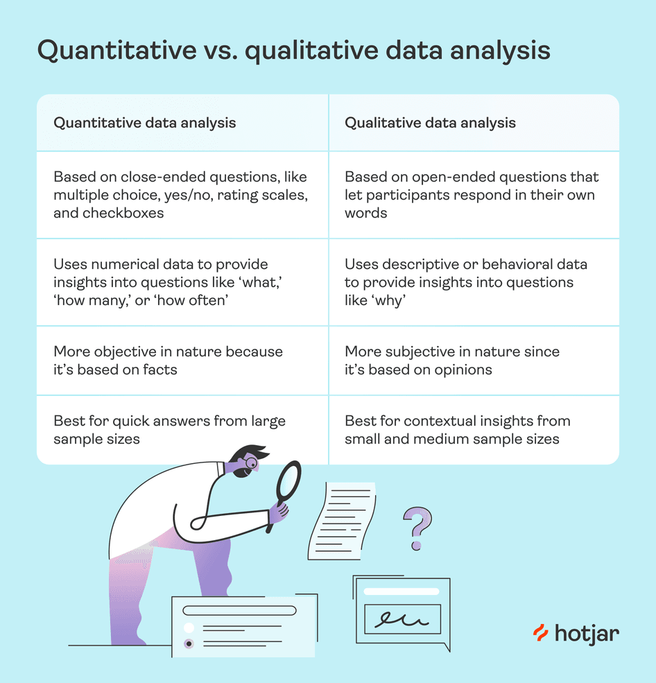
The bottom line: quantitative data analysis and qualitative data analysis are complementary processes. They work hand-in-hand to tell you what’s happening in your business and why.  

💡 Pro tip: easily toggle between quantitative and qualitative data analysis with Hotjar Funnels . 

The Funnels tool helps you visualize quantitative metrics like drop-off and conversion rates in your sales or conversion funnel to understand when and where users leave your website. You can break down your data even further to compare conversion performance by user segment.

Spot a potential issue? A single click takes you to relevant session recordings , where you see user behaviors like mouse movements, scrolls, and clicks. With this qualitative data to provide context, you'll better understand what you need to optimize to streamline the user experience (UX) and increase conversions .

Hotjar Funnels lets you quickly explore the story behind the quantitative data

4 benefits of quantitative data analysis

There’s a reason product, web design, and marketing teams take time to analyze metrics: the process pays off big time. 

Four major benefits of quantitative data analysis include:

1. Make confident decisions 

With quantitative data analysis, you know you’ve got data-driven insights to back up your decisions . For example, if you launch a concept testing survey to gauge user reactions to a new logo design, and 92% of users rate it ‘very good’—you'll feel certain when you give the designer the green light. 

Since you’re relying less on intuition and more on facts, you reduce the risks of making the wrong decision. (You’ll also find it way easier to get buy-in from team members and stakeholders for your next proposed project. 🙌)

2. Reduce costs

By crunching the numbers, you can spot opportunities to reduce spend . For example, if an ad campaign has lower-than-average click-through rates , you might decide to cut your losses and invest your budget elsewhere. 

Or, by analyzing ecommerce metrics , like website traffic by source, you may find you’re getting very little return on investment from a certain social media channel—and scale back spending in that area.

3. Personalize the user experience

Quantitative data analysis helps you map the customer journey , so you get a better sense of customers’ demographics, what page elements they interact with on your site, and where they drop off or convert . 

These insights let you better personalize your website, product, or communication, so you can segment ads, emails, and website content for specific user personas or target groups.

4. Improve user satisfaction and delight

Quantitative data analysis lets you see where your website or product is doing well—and where it falls short for your users . For example, you might see stellar results from KPIs like time on page, but conversion rates for that page are low. 

These quantitative insights encourage you to dive deeper into qualitative data to see why that’s happening—looking for moments of confusion or frustration on session recordings, for example—so you can make adjustments and optimize your conversions by improving customer satisfaction and delight.

💡Pro tip: use Net Promoter Score® (NPS) surveys to capture quantifiable customer satisfaction data that’s easy for you to analyze and interpret. 

With an NPS tool like Hotjar, you can create an on-page survey to ask users how likely they are to recommend you to others on a scale from 0 to 10. (And for added context, you can ask follow-up questions about why customers selected the rating they did—rich qualitative data is always a bonus!)

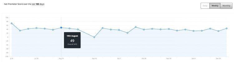
Hotjar graphs your quantitative NPS data to show changes over time

4 steps to effective quantitative data analysis 

Quantitative data analysis sounds way more intimidating than it actually is. Here’s how to make sense of your company’s numbers in just four steps:

1. Collect data

Before you can actually start the analysis process, you need data to analyze. This involves conducting quantitative research and collecting numerical data from various sources, including: 

Interviews or focus groups 

Website analytics

Observations, from tools like heatmaps or session recordings

Questionnaires, like surveys or on-page feedback widgets

Just ensure the questions you ask in your surveys are close-ended questions—providing respondents with select choices to choose from instead of open-ended questions that allow for free responses.

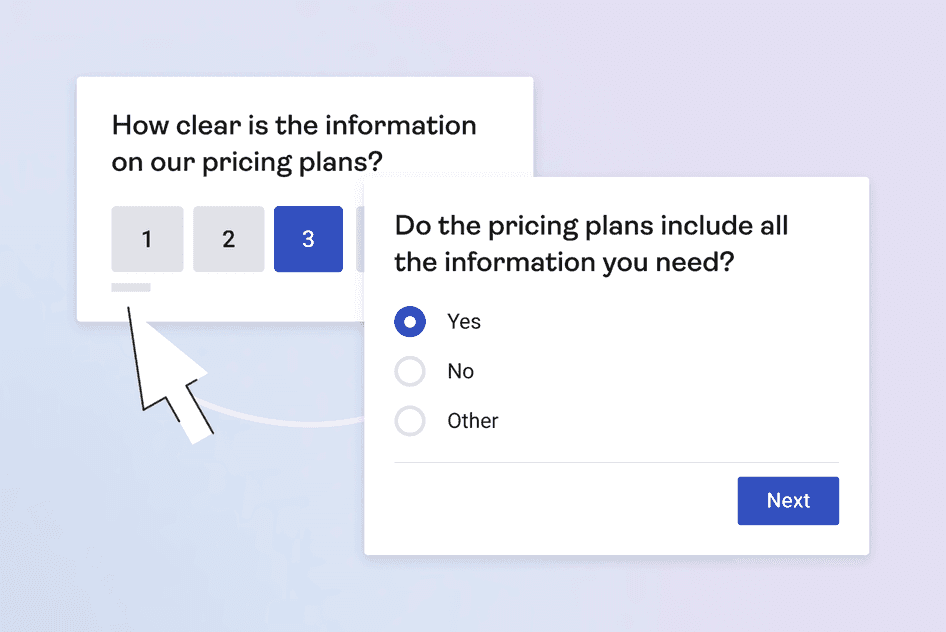
Hotjar’s pricing plans survey template provides close-ended questions

 2. Clean data

Once you’ve collected your data, it’s time to clean it up. Look through your results to find errors, duplicates, and omissions. Keep an eye out for outliers, too. Outliers are data points that differ significantly from the rest of the set—and they can skew your results if you don’t remove them.

By taking the time to clean your data set, you ensure your data is accurate, consistent, and relevant before it’s time to analyze. 

3. Analyze and interpret data

At this point, your data’s all cleaned up and ready for the main event. This step involves crunching the numbers to find patterns and trends via mathematical and statistical methods. 

Two main branches of quantitative data analysis exist: 

Descriptive analysis : methods to summarize or describe attributes of your data set. For example, you may calculate key stats like distribution and frequency, or mean, median, and mode.

Inferential analysis : methods that let you draw conclusions from statistics—like analyzing the relationship between variables or making predictions. These methods include t-tests, cross-tabulation, and factor analysis. (For more detailed explanations and how-tos, head to our guide on quantitative data analysis methods.)

Then, interpret your data to determine the best course of action. What does the data suggest you do ? For example, if your analysis shows a strong correlation between email open rate and time sent, you may explore optimal send times for each user segment.

4. Visualize and share data

Once you’ve analyzed and interpreted your data, create easy-to-read, engaging data visualizations—like charts, graphs, and tables—to present your results to team members and stakeholders. Data visualizations highlight similarities and differences between data sets and show the relationships between variables.

Software can do this part for you. For example, the Hotjar Dashboard shows all of your key metrics in one place—and automatically creates bar graphs to show how your top pages’ performance compares. And with just one click, you can navigate to the Trends tool to analyze product metrics for different segments on a single chart. 

Hotjar Trends lets you compare metrics across segments

Discover rich user insights with quantitative data analysis

Conducting quantitative data analysis takes a little bit of time and know-how, but it’s much more manageable than you might think. 

By choosing the right methods and following clear steps, you gain insights into product performance and customer experience —and you’ll be well on your way to making better decisions and creating more customer satisfaction and loyalty.

FAQs about quantitative data analysis

What is quantitative data analysis.

Quantitative data analysis is the process of making sense of numerical data through mathematical calculations and statistical tests. It helps you identify patterns, relationships, and trends to make better decisions.

How is quantitative data analysis different from qualitative data analysis?

Quantitative and qualitative data analysis are both essential processes for making sense of quantitative and qualitative research .

Quantitative data analysis helps you summarize and interpret numerical results from close-ended questions to understand what is happening. Qualitative data analysis helps you summarize and interpret non-numerical results, like opinions or behavior, to understand why the numbers look like they do.

 If you want to make strong data-driven decisions, you need both.

What are some benefits of quantitative data analysis?

Quantitative data analysis turns numbers into rich insights. Some benefits of this process include: 

Making more confident decisions

Identifying ways to cut costs

Personalizing the user experience

Improving customer satisfaction

What methods can I use to analyze quantitative data?

Quantitative data analysis has two branches: descriptive statistics and inferential statistics. 

Descriptive statistics provide a snapshot of the data’s features by calculating measures like mean, median, and mode. 

Inferential statistics , as the name implies, involves making inferences about what the data means. Dozens of methods exist for this branch of quantitative data analysis, but three commonly used techniques are: 

Cross tabulation

Factor analysis