problem solving is algorithm

What is Problem Solving Algorithm?, Steps, Representation

• Post author: Disha Singh
• Post published: 6 June 2021
• Post category: Computer Science
• Post comments: 0 Comments

Table of Contents

• 1 What is Problem Solving Algorithm?
• 2 Definition of Problem Solving Algorithm
• 3.1 Analysing the Problem
• 3.2 Developing an Algorithm
• 3.4 Testing and Debugging
• 4.1 Flowchart
• 4.2 Pseudo code

What is Problem Solving Algorithm?

Computers are used for solving various day-to-day problems and thus problem solving is an essential skill that a computer science student should know. It is pertinent to mention that computers themselves cannot solve a problem. Precise step-by-step instructions should be given by us to solve the problem.

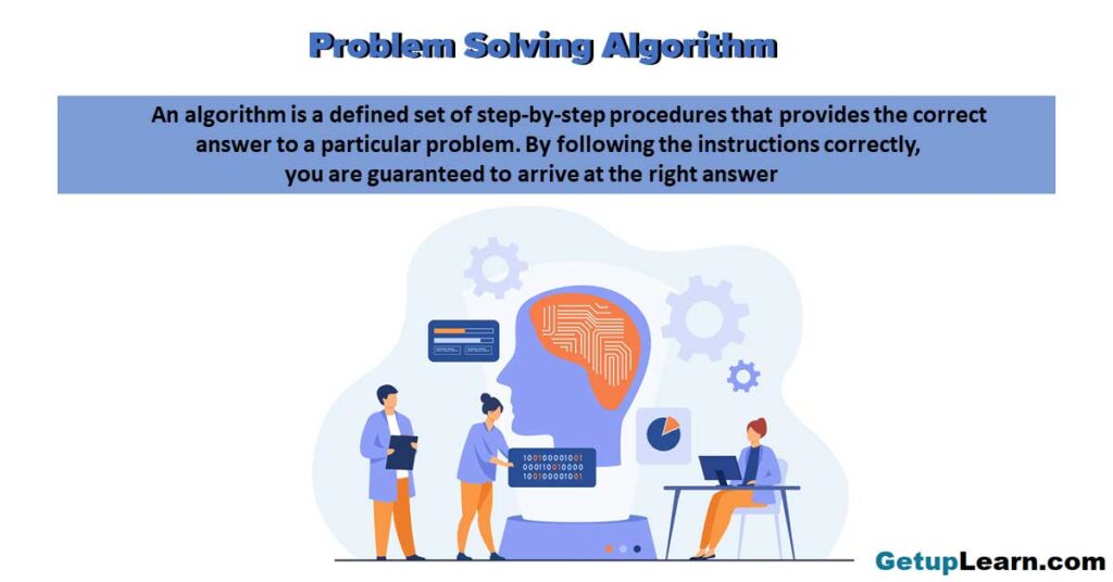
Thus, the success of a computer in solving a problem depends on how correctly and precisely we define the problem, design a solution (algorithm) and implement the solution (program) using a programming language.

Thus, problem solving is the process of identifying a problem, developing an algorithm for the identified problem and finally implementing the algorithm to develop a computer program.

Definition of Problem Solving Algorithm

These are some simple definition of problem solving algorithm which given below:

Steps for Problem Solving

When problems are straightforward and easy, we can easily find the solution. But a complex problem requires a methodical approach to find the right solution. In other words, we have to apply problem solving techniques.

Problem solving begins with the precise identification of the problem and ends with a complete working solution in terms of a program or software. Key steps required for solving a problem using a computer.

For Example: Suppose while driving, a vehicle starts making a strange noise. We might not know how to solve the problem right away. First, we need to identify from where the noise is coming? In case the problem cannot be solved by us, then we need to take the vehicle to a mechanic.

The mechanic will analyse the problem to identify the source of the noise, make a plan about the work to be done and finally repair the vehicle in order to remove the noise. From the example, it is explicit that, finding the solution to a problem might consist of multiple steps.

Following are Steps for Problem Solving :

Analysing the Problem

Developing an algorithm, testing and debugging.

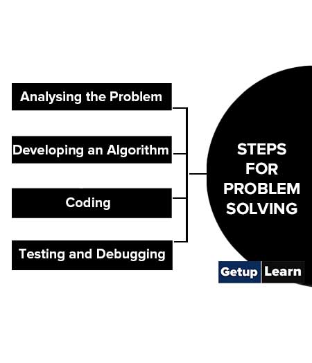
It is important to clearly understand a problem before we begin to find the solution for it. If we are not clear as to what is to be solved, we may end up developing a program which may not solve our purpose.

Thus, we need to read and analyse the problem statement carefully in order to list the principal components of the problem and decide the core functionalities that our solution should have. By analysing a problem, we would be able to figure out what are the inputs that our program should accept and the outputs that it should produce.

It is essential to device a solution before writing a program code for a given problem. The solution is represented in natural language and is called an algorithm. We can imagine an algorithm like a very well-written recipe for a dish, with clearly defined steps that, if followed, one will end up preparing the dish.

We start with a tentative solution plan and keep on refining the algorithm until the algorithm is able to capture all the aspects of the desired solution. For a given problem, more than one algorithm is possible and we have to select the most suitable solution.

After finalising the algorithm, we need to convert the algorithm into the format which can be understood by the computer to generate the desired solution. Different high level programming languages can be used for writing a program. It is equally important to record the details of the coding procedures followed and document the solution. This is helpful when revisiting the programs at a later stage.

The program created should be tested on various parameters. The program should meet the requirements of the user. It must respond within the expected time. It should generate correct output for all possible inputs. In the presence of syntactical errors, no output will be obtained. In case the output generated is incorrect, then the program should be checked for logical errors, if any.

Software industry follows standardised testing methods like unit or component testing, integration testing, system testing, and acceptance testing while developing complex applications. This is to ensure that the software meets all the business and technical requirements and works as expected.

The errors or defects found in the testing phases are debugged or rectified and the program is again tested. This continues till all the errors are removed from the program. Once the software application has been developed, tested and delivered to the user, still problems in terms of functioning can come up and need to be resolved from time to time.

The maintenance of the solution, thus, involves fixing the problems faced by the user, answering the queries of the user and even serving the request for addition or modification of features.

Representation of Algorithms

Using their algorithmic thinking skills, the software designers or programmers analyse the problem and identify the logical steps that need to be followed to reach a solution. Once the steps are identified, the need is to write down these steps along with the required input and desired output.

There are two common methods of representing an algorithm —flowchart and pseudocode. Either of the methods can be used to represent an algorithm while keeping in mind the following:

• It showcases the logic of the problem solution, excluding any implementational details.
• It clearly reveals the flow of control during execution of the program.

A flowchart is a visual representation of an algorithm . A flowchart is a diagram made up of boxes, diamonds and other shapes, connected by arrows. Each shape represents a step of the solution process and the arrow represents the order or link among the steps.

A flow chart is a step by step diagrammatic representation of the logic paths to solve a given problem. Or A flowchart is visual or graphical representation of an algorithm .

The flowcharts are pictorial representation of the methods to b used to solve a given problem and help a great deal to analyze the problem and plan its solution in a systematic and orderly manner. A flowchart when translated in to a proper computer language, results in a complete program.

Advantages of Flowcharts:

• The flowchart shows the logic of a problem displayed in pictorial fashion which felicitates easier checking of an algorithm
• The Flowchart is good means of communication to other users. It is also a compact means of recording an algorithm solution to a problem.
• The flowchart allows the problem solver to break the problem into parts. These parts can be connected to make master chart.
• The flowchart is a permanent record of the solution which can be consulted at a later time.

Differences between Algorithm and Flowchart

Pseudo code.

The Pseudo code is neither an algorithm nor a program. It is an abstract form of a program. It consists of English like statements which perform the specific operations. It is defined for an algorithm. It does not use any graphical representation.

In pseudo code , the program is represented in terms of words and phrases, but the syntax of program is not strictly followed.

Advantages of Pseudocode

• Before writing codes in a high level language, a pseudocode of a program helps in representing the basic functionality of the intended program.
• By writing the code first in a human readable language, the programmer safeguards against leaving out any important step. Besides, for non-programmers, actual programs are difficult to read and understand.
• But pseudocode helps them to review the steps to confirm that the proposed implementation is going to achieve the desire output.

Related posts:

10 Types of Computers | History of Computers, Advantages

What is microprocessor evolution of microprocessor, types, features, types of computer memory, characteristics, primary memory, secondary memory, data and information: definition, characteristics, types, channels, approaches, what is cloud computing classification, characteristics, principles, types of cloud providers, what is debugging types of errors, types of storage devices, advantages, examples, 10 evolution of computing machine, history, what are functions of operating system 6 functions, advantages and disadvantages of operating system, data representation in computer: number systems, characters, audio, image and video.

• What are Data Types in C++? Types

What are Operators in C? Different Types of Operators in C

• What are Expressions in C? Types

What are Decision Making Statements in C? Types

You might also like.

What is C++ Programming Language? C++ Character Set, C++ Tokens

What is Artificial Intelligence? Functions, 6 Benefits, Applications of AI

What is Computer System? Definition, Characteristics, Functional Units, Components

What is Big Data? Characteristics, Tools, Types, Internet of Things (IOT)

Advantages and Disadvantages of Flowcharts

Generations of Computer First To Fifth, Classification, Characteristics, Features, Examples

What is operating system? Functions, Types, Types of User Interface

• Entrepreneurship
• Organizational Behavior
• Financial Management
• Communication
• Human Resource Management
• Sales Management
• Marketing Management

• Admiral “Amazing Grace” Hopper

Exploring the Intricacies of NP-Completeness in Computer Science

Understanding p vs np problems in computer science: a primer for beginners, understanding key theoretical frameworks in computer science: a beginner’s guide.

Learn Computer Science with Python

CS is a journey, not a destination

• Foundations

Understanding Algorithms: The Key to Problem-Solving Mastery

The world of computer science is a fascinating realm, where intricate concepts and technologies continuously shape the way we interact with machines. Among the vast array of ideas and principles, few are as fundamental and essential as algorithms. These powerful tools serve as the building blocks of computation, enabling computers to solve problems, make decisions, and process vast amounts of data efficiently.

An algorithm can be thought of as a step-by-step procedure or a set of instructions designed to solve a specific problem or accomplish a particular task. It represents a systematic approach to finding solutions and provides a structured way to tackle complex computational challenges. Algorithms are at the heart of various applications, from simple calculations to sophisticated machine learning models and complex data analysis.

Understanding algorithms and their inner workings is crucial for anyone interested in computer science. They serve as the backbone of software development, powering the creation of innovative applications across numerous domains. By comprehending the concept of algorithms, aspiring computer science enthusiasts gain a powerful toolset to approach problem-solving and gain insight into the efficiency and performance of different computational methods.

In this article, we aim to provide a clear and accessible introduction to algorithms, focusing on their importance in problem-solving and exploring common types such as searching, sorting, and recursion. By delving into these topics, readers will gain a solid foundation in algorithmic thinking and discover the underlying principles that drive the functioning of modern computing systems. Whether you’re a beginner in the world of computer science or seeking to deepen your understanding, this article will equip you with the knowledge to navigate the fascinating world of algorithms.

What are Algorithms?

At its core, an algorithm is a systematic, step-by-step procedure or set of rules designed to solve a problem or perform a specific task. It provides clear instructions that, when followed meticulously, lead to the desired outcome.

Consider an algorithm to be akin to a recipe for your favorite dish. When you decide to cook, the recipe is your go-to guide. It lists out the ingredients you need, their exact quantities, and a detailed, step-by-step explanation of the process, from how to prepare the ingredients to how to mix them, and finally, the cooking process. It even provides an order for adding the ingredients and specific times for cooking to ensure the dish turns out perfect.

In the same vein, an algorithm, within the realm of computer science, provides an explicit series of instructions to accomplish a goal. This could be a simple goal like sorting a list of numbers in ascending order, a more complex task such as searching for a specific data point in a massive dataset, or even a highly complicated task like determining the shortest path between two points on a map (think Google Maps). No matter the complexity of the problem at hand, there’s always an algorithm working tirelessly behind the scenes to solve it.

Furthermore, algorithms aren’t limited to specific programming languages. They are universal and can be implemented in any language. This is why understanding the fundamental concept of algorithms can empower you to solve problems across various programming languages.

The Importance of Algorithms

Algorithms are indisputably the backbone of all computational operations. They’re a fundamental part of the digital world that we interact with daily. When you search for something on the web, an algorithm is tirelessly working behind the scenes to sift through millions, possibly billions, of web pages to bring you the most relevant results. When you use a GPS to find the fastest route to a location, an algorithm is computing all possible paths, factoring in variables like traffic and road conditions, to provide you the optimal route.

Consider the world of social media, where algorithms curate personalized feeds based on our previous interactions, or in streaming platforms where they recommend shows and movies based on our viewing habits. Every click, every like, every search, and every interaction is processed by algorithms to serve you a seamless digital experience.

In the realm of computer science and beyond, everything revolves around problem-solving, and algorithms are our most reliable problem-solving tools. They provide a structured approach to problem-solving, breaking down complex problems into manageable steps and ensuring that every eventuality is accounted for.

Moreover, an algorithm’s efficiency is not just a matter of preference but a necessity. Given that computers have finite resources — time, memory, and computational power — the algorithms we use need to be optimized to make the best possible use of these resources. Efficient algorithms are the ones that can perform tasks more quickly, using less memory, and provide solutions to complex problems that might be infeasible with less efficient alternatives.

In the context of massive datasets (the likes of which are common in our data-driven world), the difference between a poorly designed algorithm and an efficient one could be the difference between a solution that takes years to compute and one that takes mere seconds. Therefore, understanding, designing, and implementing efficient algorithms is a critical skill for any computer scientist or software engineer.

Hence, as a computer science beginner, you are starting a journey where algorithms will be your best allies — universal keys capable of unlocking solutions to a myriad of problems, big or small.

Common Types of Algorithms: Searching and Sorting

Two of the most ubiquitous types of algorithms that beginners often encounter are searching and sorting algorithms.

Searching algorithms are designed to retrieve specific information from a data structure, like an array or a database. A simple example is the linear search, which works by checking each element in the array until it finds the one it’s looking for. Although easy to understand, this method isn’t efficient for large datasets, which is where more complex algorithms like binary search come in.

Binary search, on the other hand, is like looking up a word in the dictionary. Instead of checking each word from beginning to end, you open the dictionary in the middle and see if the word you’re looking for should be on the left or right side, thereby reducing the search space by half with each step.

Sorting algorithms, meanwhile, are designed to arrange elements in a particular order. A simple sorting algorithm is bubble sort, which works by repeatedly swapping adjacent elements if they’re in the wrong order. Again, while straightforward, it’s not efficient for larger datasets. More advanced sorting algorithms, such as quicksort or mergesort, have been designed to sort large data collections more efficiently.

Diving Deeper: Graph and Dynamic Programming Algorithms

Building upon our understanding of searching and sorting algorithms, let’s delve into two other families of algorithms often encountered in computer science: graph algorithms and dynamic programming algorithms.

A graph is a mathematical structure that models the relationship between pairs of objects. Graphs consist of vertices (or nodes) and edges (where each edge connects a pair of vertices). Graphs are commonly used to represent real-world systems such as social networks, web pages, biological networks, and more.

Graph algorithms are designed to solve problems centered around these structures. Some common graph algorithms include:

Dynamic programming is a powerful method used in optimization problems, where the main problem is broken down into simpler, overlapping subproblems. The solutions to these subproblems are stored and reused to build up the solution to the main problem, saving computational effort.

Here are two common dynamic programming problems:

Understanding these algorithm families — searching, sorting, graph, and dynamic programming algorithms — not only equips you with powerful tools to solve a variety of complex problems but also serves as a springboard to dive deeper into the rich ocean of algorithms and computer science.

Recursion: A Powerful Technique

While searching and sorting represent specific problem domains, recursion is a broad technique used in a wide range of algorithms. Recursion involves breaking down a problem into smaller, more manageable parts, and a function calling itself to solve these smaller parts.

To visualize recursion, consider the task of calculating factorial of a number. The factorial of a number n (denoted as n! ) is the product of all positive integers less than or equal to n . For instance, the factorial of 5 ( 5! ) is 5 x 4 x 3 x 2 x 1 = 120 . A recursive algorithm for finding factorial of n would involve multiplying n by the factorial of n-1 . The function keeps calling itself with a smaller value of n each time until it reaches a point where n is equal to 1, at which point it starts returning values back up the chain.

Algorithms are truly the heart of computer science, transforming raw data into valuable information and insight. Understanding their functionality and purpose is key to progressing in your computer science journey. As you continue your exploration, remember that each algorithm you encounter, no matter how complex it may seem, is simply a step-by-step procedure to solve a problem.

We’ve just scratched the surface of the fascinating world of algorithms. With time, patience, and practice, you will learn to create your own algorithms and start solving problems with confidence and efficiency.

Related Articles

Three Elegant Algorithms Every Computer Science Beginner Should Know

What is an Algorithm? Algorithm Definition for Computer Science Beginners

If you’re a student and want to study computer science, or you’re learning to code, then there’s a chance you’ve heard of algorithms. Simply put, an algorithm is a set of instructions that performs a particular action.

Contrary to popular belief, an algorithm is not some piece of code that requires extremely advanced knowledge in order to implement. At the same time, I won't say that an algorithm is easy to implement, either. Some can be, but it depends on what you're trying to do.

In the end, the best way to get better at algorithms is by practicing them regularly.

In this article, you'll learn all about algorithms so you'll be prepared next time you encounter one, or have to write one yourself. I will also share some freeCodeCamp resources that will help you learn how to write algorithms in different languages.

What We'll Cover

What exactly is an algorithm.

• Why Do You Need an Algorithm?

Types of Algorithms

• Which Programming Language Is Best for Writing Algorithms? (rename)

Resources for Learning Algorithms

An algorithm is a set of steps for solving a known problem. Most algorithms are implemented to run following the four steps below:

• take an input
• access that input and make sure it's correct
• show the result
• terminate (the stage where the algorithm stop running)

Some steps of the algorithm may run repeatedly, but in the end, termination is what ends an algorithm.

For example, the algorithm below sort numbers in descending order. It loops through the numbers specified until it arranges them in descending order, then terminates when there are no more number to sort:

For a theoretical basis, for instance, an algorithm for dividing two numbers and showing the remainder could run through the steps below:

• Step 1 : the user enters the first and second numbers – the dividend and the divisor
• Step 2 : the algorithm written to perform the division takes in the number, then puts a division sign between the dividend and the divisor. It also checks for a remainder.
• Step 3 : the result of the division and remainder is shown to the user
• Step 4 : the algorithm terminates

Here's how that kind of algorithm is implemented in JavaScript:

If there's an error, the algorithm may not run, or might return the wrong output. If the programmer who wrote the algorithm took user experience into consideration, then an error handler could show an error to the user and let them know what to do.

Why do you Need an Algorithm?

If you’re one of those computer science students asking “why algorithms”, here are some reasons why you should learn about them:

Problem Solving : being able to write an algorithm improves your problem-solving capacity. It is a common belief that once you can solve a problem with one thing, you can solve problems with another closely related one. So, if you can solve problems with Python, you can solve problems with JavaScript.

Scalability : an algorithm helps your software/application/website respond appropriately to demands.

Proper Utilization of Resources: choosing the right algorithm ensures proper utilization of resources such as memory, storage, network, and others.

Algorithms in computer science can be broadly categorized into searching and sorting algorithms:

• Sorting – selection sort, bubble sort, insertion sort, merge sort, quick sort, and so on.
• Searching – binary search, exponential search, jump search, and so on.

But there are many types of algorithms that programers use regularly. Here are some other common algorithm types organized by category:

• Hashing – SHA-256, SHA-1
• Brute force – trial and error
• Divide and conquer – merge sort algorithm
• Greedy – Prim's algorithm, Kruskal's algorithm
• Recursive – computer factorials

Which Programming Language Is Best for Writing Algorithms?

You can write angorithms in any programming language. There's no benefit to using one language over another.

Every language has its strengths and weaknesses, and each has unique syntax and features. So writing an algorithm might look different in one language compared to another.

But algorithms are universal concepts. So if you can write bubble sort in Python, you should also be able to write it in JavaScript or C#.

Here are some videos from the freeCodeCamp YouTube channel that can help you learn algorithms effectively:

• Algorithms and Data Structures Tutorial - Full Course for Beginners
• Algorithms in Python – Full Course for Beginners
• Data Structures Easy to Advanced Course - Full Tutorial from a Google Engineer
• Dynamic Programming - Learn to Solve Algorithmic Problems & Coding Challenges
• Understanding Sorting Algorithms

Also, the interactive JavaScript Algorithms and Data Structures Certification on freeCodeCamp can give you a crash course in algorithmic thinking in JavaScript.

In this article, we went over what an algorithm is, their types, and resources for learning algorithms.

If you read this far, the next thing you should do is start learning algorithms with one or more of the resources listed in this article.

Thank you for reading.

Web developer and technical writer focusing on frontend technologies. I also dabble in a lot of other technologies.

If you read this far, thank the author to show them you care. Say Thanks

Learn to code for free. freeCodeCamp's open source curriculum has helped more than 40,000 people get jobs as developers. Get started

Smart. Open. Grounded. Inventive. Read our Ideas Made to Matter.

Which program is right for you?

Through intellectual rigor and experiential learning, this full-time, two-year MBA program develops leaders who make a difference in the world.

A rigorous, hands-on program that prepares adaptive problem solvers for premier finance careers.

A 12-month program focused on applying the tools of modern data science, optimization and machine learning to solve real-world business problems.

Earn your MBA and SM in engineering with this transformative two-year program.

Combine an international MBA with a deep dive into management science. A special opportunity for partner and affiliate schools only.

A doctoral program that produces outstanding scholars who are leading in their fields of research.

Bring a business perspective to your technical and quantitative expertise with a bachelor’s degree in management, business analytics, or finance.

A joint program for mid-career professionals that integrates engineering and systems thinking. Earn your master’s degree in engineering and management.

An interdisciplinary program that combines engineering, management, and design, leading to a master’s degree in engineering and management.

Executive Programs

A full-time MBA program for mid-career leaders eager to dedicate one year of discovery for a lifetime of impact.

This 20-month MBA program equips experienced executives to enhance their impact on their organizations and the world.

Non-degree programs for senior executives and high-potential managers.

A non-degree, customizable program for mid-career professionals.

Women’s career advice: Remember that exhaustion is not a yardstick for productivity

How, and why, to run a values-based business

Accelerated research about generative AI

Credit: Alejandro Giraldo

Ideas Made to Matter

How to use algorithms to solve everyday problems

Kara Baskin

May 8, 2017

How can I navigate the grocery store quickly? Why doesn’t anyone like my Facebook status? How can I alphabetize my bookshelves in a hurry? Apple data visualizer and MIT System Design and Management graduate Ali Almossawi solves these common dilemmas and more in his new book, “ Bad Choices: How Algorithms Can Help You Think Smarter and Live Happier ,” a quirky, illustrated guide to algorithmic thinking. 

For the uninitiated: What is an algorithm? And how can algorithms help us to think smarter?

An algorithm is a process with unambiguous steps that has a beginning and an end, and does something useful.

Algorithmic thinking is taking a step back and asking, “If it’s the case that algorithms are so useful in computing to achieve predictability, might they also be useful in everyday life, when it comes to, say, deciding between alternative ways of solving a problem or completing a task?” In all cases, we optimize for efficiency: We care about time or space.

Note the mention of “deciding between.” Computer scientists do that all the time, and I was convinced that the tools they use to evaluate competing algorithms would be of interest to a broad audience.

Why did you write this book, and who can benefit from it?

All the books I came across that tried to introduce computer science involved coding. My approach to making algorithms compelling was focusing on comparisons. I take algorithms and put them in a scene from everyday life, such as matching socks from a pile, putting books on a shelf, remembering things, driving from one point to another, or cutting an onion. These activities can be mapped to one or more fundamental algorithms, which form the basis for the field of computing and have far-reaching applications and uses.

I wrote the book with two audiences in mind. One, anyone, be it a learner or an educator, who is interested in computer science and wants an engaging and lighthearted, but not a dumbed-down, introduction to the field. Two, anyone who is already familiar with the field and wants to experience a way of explaining some of the fundamental concepts in computer science differently than how they’re taught.

I’m going to the grocery store and only have 15 minutes. What do I do?

Do you know what the grocery store looks like ahead of time? If you know what it looks like, it determines your list. How do you prioritize things on your list? Order the items in a way that allows you to avoid walking down the same aisles twice.

For me, the intriguing thing is that the grocery store is a scene from everyday life that I can use as a launch pad to talk about various related topics, like priority queues and graphs and hashing. For instance, what is the most efficient way for a machine to store a prioritized list, and what happens when the equivalent of you scratching an item from a list happens in the machine’s list? How is a store analogous to a graph (an abstraction in computer science and mathematics that defines how things are connected), and how is navigating the aisles in a store analogous to traversing a graph?

Nobody follows me on Instagram. How do I get more followers?

The concept of links and networks, which I cover in Chapter 6, is relevant here. It’s much easier to get to people whom you might be interested in and who might be interested in you if you can start within the ball of links that connects those people, rather than starting at a random spot.

You mention Instagram: There, the hashtag is one way to enter that ball of links. Tag your photos, engage with users who tag their photos with the same hashtags, and you should be on your way to stardom.

What are the secret ingredients of a successful Facebook post?

I’ve posted things on social media that have died a sad death and then posted the same thing at a later date that somehow did great. Again, if we think of it in terms that are relevant to algorithms, we’d say that the challenge with making something go viral is really getting that first spark. And to get that first spark, a person who is connected to the largest number of people who are likely to engage with that post, needs to share it.

With [my first book], “Bad Arguments,” I spent a month pouring close to $5,000 into advertising for that project with moderate results. And then one science journalist with a large audience wrote about it, and the project took off and hasn’t stopped since.

What problems do you wish you could solve via algorithm but can’t?

When we care about efficiency, thinking in terms of algorithms is useful. There are cases when that’s not the quality we want to optimize for — for instance, learning or love. I walk for several miles every day, all throughout the city, as I find it relaxing. I’ve never asked myself, “What’s the most efficient way I can traverse the streets of San Francisco?” It’s not relevant to my objective.

Algorithms are a great way of thinking about efficiency, but the question has to be, “What approach can you optimize for that objective?” That’s what worries me about self-help: Books give you a silver bullet for doing everything “right” but leave out all the nuances that make us different. What works for you might not work for me.

Which companies use algorithms well?

When you read that the overwhelming majority of the shows that users of, say, Netflix, watch are due to Netflix’s recommendation engine, you know they’re doing something right.

Related Articles

• 1. Micro-Worlds
• 2. Light-Bot in Java
• 3. Jeroos of Santong Island
• 4. Problem Solving and Algorithms
• 5. Creating Jeroo Methods
• 6. Conditionally Executing Actions
• 7. Repeating Actions
• 8. Handling Touch Events
• 9. Adding Text to the Screen

Problem Solving and Algorithms

Learn a basic process for developing a solution to a problem. Nothing in this chapter is unique to using a computer to solve a problem. This process can be used to solve a wide variety of problems, including ones that have nothing to do with computers.

Problems, Solutions, and Tools

I have a problem! I need to thank Aunt Kay for the birthday present she sent me. I could send a thank you note through the mail. I could call her on the telephone. I could send her an email message. I could drive to her house and thank her in person. In fact, there are many ways I could thank her, but that's not the point. The point is that I must decide how I want to solve the problem, and use the appropriate tool to implement (carry out) my plan. The postal service, the telephone, the internet, and my automobile are tools that I can use, but none of these actually solves my problem. In a similar way, a computer does not solve problems, it's just a tool that I can use to implement my plan for solving the problem.

Knowing that Aunt Kay appreciates creative and unusual things, I have decided to hire a singing messenger to deliver my thanks. In this context, the messenger is a tool, but one that needs instructions from me. I have to tell the messenger where Aunt Kay lives, what time I would like the message to be delivered, and what lyrics I want sung. A computer program is similar to my instructions to the messenger.

The story of Aunt Kay uses a familiar context to set the stage for a useful point of view concerning computers and computer programs. The following list summarizes the key aspects of this point of view.

A computer is a tool that can be used to implement a plan for solving a problem.

A computer program is a set of instructions for a computer. These instructions describe the steps that the computer must follow to implement a plan.

An algorithm is a plan for solving a problem.

A person must design an algorithm.

A person must translate an algorithm into a computer program.

This point of view sets the stage for a process that we will use to develop solutions to Jeroo problems. The basic process is important because it can be used to solve a wide variety of problems, including ones where the solution will be written in some other programming language.

An Algorithm Development Process

Every problem solution starts with a plan. That plan is called an algorithm.

There are many ways to write an algorithm. Some are very informal, some are quite formal and mathematical in nature, and some are quite graphical. The instructions for connecting a DVD player to a television are an algorithm. A mathematical formula such as πR 2 is a special case of an algorithm. The form is not particularly important as long as it provides a good way to describe and check the logic of the plan.

The development of an algorithm (a plan) is a key step in solving a problem. Once we have an algorithm, we can translate it into a computer program in some programming language. Our algorithm development process consists of five major steps.

Step 1: Obtain a description of the problem.

Step 2: analyze the problem., step 3: develop a high-level algorithm., step 4: refine the algorithm by adding more detail., step 5: review the algorithm..

This step is much more difficult than it appears. In the following discussion, the word client refers to someone who wants to find a solution to a problem, and the word developer refers to someone who finds a way to solve the problem. The developer must create an algorithm that will solve the client's problem.

The client is responsible for creating a description of the problem, but this is often the weakest part of the process. It's quite common for a problem description to suffer from one or more of the following types of defects: (1) the description relies on unstated assumptions, (2) the description is ambiguous, (3) the description is incomplete, or (4) the description has internal contradictions. These defects are seldom due to carelessness by the client. Instead, they are due to the fact that natural languages (English, French, Korean, etc.) are rather imprecise. Part of the developer's responsibility is to identify defects in the description of a problem, and to work with the client to remedy those defects.

The purpose of this step is to determine both the starting and ending points for solving the problem. This process is analogous to a mathematician determining what is given and what must be proven. A good problem description makes it easier to perform this step.

When determining the starting point, we should start by seeking answers to the following questions:

What data are available?

Where is that data?

What formulas pertain to the problem?

What rules exist for working with the data?

What relationships exist among the data values?

When determining the ending point, we need to describe the characteristics of a solution. In other words, how will we know when we're done? Asking the following questions often helps to determine the ending point.

What new facts will we have?

What items will have changed?

What changes will have been made to those items?

What things will no longer exist?

An algorithm is a plan for solving a problem, but plans come in several levels of detail. It's usually better to start with a high-level algorithm that includes the major part of a solution, but leaves the details until later. We can use an everyday example to demonstrate a high-level algorithm.

Problem: I need a send a birthday card to my brother, Mark.

Analysis: I don't have a card. I prefer to buy a card rather than make one myself.

High-level algorithm:

Go to a store that sells greeting cards Select a card Purchase a card Mail the card

This algorithm is satisfactory for daily use, but it lacks details that would have to be added were a computer to carry out the solution. These details include answers to questions such as the following.

"Which store will I visit?"

"How will I get there: walk, drive, ride my bicycle, take the bus?"

"What kind of card does Mark like: humorous, sentimental, risqué?"

These kinds of details are considered in the next step of our process.

A high-level algorithm shows the major steps that need to be followed to solve a problem. Now we need to add details to these steps, but how much detail should we add? Unfortunately, the answer to this question depends on the situation. We have to consider who (or what) is going to implement the algorithm and how much that person (or thing) already knows how to do. If someone is going to purchase Mark's birthday card on my behalf, my instructions have to be adapted to whether or not that person is familiar with the stores in the community and how well the purchaser known my brother's taste in greeting cards.

When our goal is to develop algorithms that will lead to computer programs, we need to consider the capabilities of the computer and provide enough detail so that someone else could use our algorithm to write a computer program that follows the steps in our algorithm. As with the birthday card problem, we need to adjust the level of detail to match the ability of the programmer. When in doubt, or when you are learning, it is better to have too much detail than to have too little.

Most of our examples will move from a high-level to a detailed algorithm in a single step, but this is not always reasonable. For larger, more complex problems, it is common to go through this process several times, developing intermediate level algorithms as we go. Each time, we add more detail to the previous algorithm, stopping when we see no benefit to further refinement. This technique of gradually working from a high-level to a detailed algorithm is often called stepwise refinement .

The final step is to review the algorithm. What are we looking for? First, we need to work through the algorithm step by step to determine whether or not it will solve the original problem. Once we are satisfied that the algorithm does provide a solution to the problem, we start to look for other things. The following questions are typical of ones that should be asked whenever we review an algorithm. Asking these questions and seeking their answers is a good way to develop skills that can be applied to the next problem.

Does this algorithm solve a very specific problem or does it solve a more general problem ? If it solves a very specific problem, should it be generalized?

For example, an algorithm that computes the area of a circle having radius 5.2 meters (formula π*5.2 2 ) solves a very specific problem, but an algorithm that computes the area of any circle (formula π*R 2 ) solves a more general problem.

Can this algorithm be simplified ?

One formula for computing the perimeter of a rectangle is:

length + width + length + width

A simpler formula would be:

2.0 * ( length + width )

Is this solution similar to the solution to another problem? How are they alike? How are they different?

For example, consider the following two formulae:

Rectangle area = length * width Triangle area = 0.5 * base * height

Similarities: Each computes an area. Each multiplies two measurements.

Differences: Different measurements are used. The triangle formula contains 0.5.

Hypothesis: Perhaps every area formula involves multiplying two measurements.

Example 4.1: Pick and Plant

This section contains an extended example that demonstrates the algorithm development process. To complete the algorithm, we need to know that every Jeroo can hop forward, turn left and right, pick a flower from its current location, and plant a flower at its current location.

Problem Statement (Step 1)

A Jeroo starts at (0, 0) facing East with no flowers in its pouch. There is a flower at location (3, 0). Write a program that directs the Jeroo to pick the flower and plant it at location (3, 2). After planting the flower, the Jeroo should hop one space East and stop. There are no other nets, flowers, or Jeroos on the island.

Analysis of the Problem (Step 2)

The flower is exactly three spaces ahead of the jeroo.

The flower is to be planted exactly two spaces South of its current location.

The Jeroo is to finish facing East one space East of the planted flower.

There are no nets to worry about.

High-level Algorithm (Step 3)

Let's name the Jeroo Bobby. Bobby should do the following:

Get the flower Put the flower Hop East

Detailed Algorithm (Step 4)

Get the flower Hop 3 times Pick the flower Put the flower Turn right Hop 2 times Plant a flower Hop East Turn left Hop once

Review the Algorithm (Step 5)

The high-level algorithm partitioned the problem into three rather easy subproblems. This seems like a good technique.

This algorithm solves a very specific problem because the Jeroo and the flower are in very specific locations.

This algorithm is actually a solution to a slightly more general problem in which the Jeroo starts anywhere, and the flower is 3 spaces directly ahead of the Jeroo.

Java Code for "Pick and Plant"

A good programmer doesn't write a program all at once. Instead, the programmer will write and test the program in a series of builds. Each build adds to the previous one. The high-level algorithm will guide us in this process.

FIRST BUILD

To see this solution in action, create a new Greenfoot4Sofia scenario and use the Edit Palettes Jeroo menu command to make the Jeroo classes visible. Right-click on the Island class and create a new subclass with the name of your choice. This subclass will hold your new code.

The recommended first build contains three things:

The main method (here myProgram() in your island subclass).

Declaration and instantiation of every Jeroo that will be used.

The high-level algorithm in the form of comments.

The instantiation at the beginning of myProgram() places bobby at (0, 0), facing East, with no flowers.

Once the first build is working correctly, we can proceed to the others. In this case, each build will correspond to one step in the high-level algorithm. It may seem like a lot of work to use four builds for such a simple program, but doing so helps establish habits that will become invaluable as the programs become more complex.

SECOND BUILD

This build adds the logic to "get the flower", which in the detailed algorithm (step 4 above) consists of hopping 3 times and then picking the flower. The new code is indicated by comments that wouldn't appear in the original (they are just here to call attention to the additions). The blank lines help show the organization of the logic.

By taking a moment to run the work so far, you can confirm whether or not this step in the planned algorithm works as expected.

THIRD BUILD

This build adds the logic to "put the flower". New code is indicated by the comments that are provided here to mark the additions.

FOURTH BUILD (final)

Example 4.2: replace net with flower.

This section contains a second example that demonstrates the algorithm development process.

There are two Jeroos. One Jeroo starts at (0, 0) facing North with one flower in its pouch. The second starts at (0, 2) facing East with one flower in its pouch. There is a net at location (3, 2). Write a program that directs the first Jeroo to give its flower to the second one. After receiving the flower, the second Jeroo must disable the net, and plant a flower in its place. After planting the flower, the Jeroo must turn and face South. There are no other nets, flowers, or Jeroos on the island.

Jeroo_2 is exactly two spaces behind Jeroo_1.

The only net is exactly three spaces ahead of Jeroo_2.

Each Jeroo has exactly one flower.

Jeroo_2 will have two flowers after receiving one from Jeroo_1. One flower must be used to disable the net. The other flower must be planted at the location of the net, i.e. (3, 2).

Jeroo_1 will finish at (0, 1) facing South.

Jeroo_2 is to finish at (3, 2) facing South.

Each Jeroo will finish with 0 flowers in its pouch. One flower was used to disable the net, and the other was planted.

Let's name the first Jeroo Ann and the second one Andy.

Ann should do the following: Find Andy (but don't collide with him) Give a flower to Andy (he will be straight ahead) After receiving the flower, Andy should do the following: Find the net (but don't hop onto it) Disable the net Plant a flower at the location of the net Face South

Ann should do the following: Find Andy Turn around (either left or right twice) Hop (to location (0, 1)) Give a flower to Andy Give ahead Now Andy should do the following: Find the net Hop twice (to location (2, 2)) Disable the net Toss Plant a flower at the location of the net Hop (to location (3, 2)) Plant a flower Face South Turn right

The high-level algorithm helps manage the details.

This algorithm solves a very specific problem, but the specific locations are not important. The only thing that is important is the starting location of the Jeroos relative to one another and the location of the net relative to the second Jeroo's location and direction.

Java Code for "Replace Net with Flower"

As before, the code should be written incrementally as a series of builds. Four builds will be suitable for this problem. As usual, the first build will contain the main method, the declaration and instantiation of the Jeroo objects, and the high-level algorithm in the form of comments. The second build will have Ann give her flower to Andy. The third build will have Andy locate and disable the net. In the final build, Andy will place the flower and turn East.

This build creates the main method, instantiates the Jeroos, and outlines the high-level algorithm. In this example, the main method would be myProgram() contained within a subclass of Island .

This build adds the logic for Ann to locate Andy and give him a flower.

This build adds the logic for Andy to locate and disable the net.

This build adds the logic for Andy to place a flower at (3, 2) and turn South.

If you're seeing this message, it means we're having trouble loading external resources on our website.

If you're behind a web filter, please make sure that the domains *.kastatic.org and *.kasandbox.org are unblocked.

To log in and use all the features of Khan Academy, please enable JavaScript in your browser.

Unit 1: Algorithms

About this unit.

We've partnered with Dartmouth college professors Tom Cormen and Devin Balkcom to teach introductory computer science algorithms, including searching, sorting, recursion, and graph theory. Learn with a combination of articles, visualizations, quizzes, and coding challenges.

Intro to algorithms

• What is an algorithm and why should you care? (Opens a modal)
• A guessing game (Opens a modal)
• Route-finding (Opens a modal)
• Discuss: Algorithms in your life (Opens a modal)

Binary search

• Binary search (Opens a modal)
• Implementing binary search of an array (Opens a modal)
• Challenge: Binary search (Opens a modal)
• Running time of binary search (Opens a modal)
• Running time of binary search 5 questions Practice

Asymptotic notation

• Asymptotic notation (Opens a modal)
• Big-θ (Big-Theta) notation (Opens a modal)
• Functions in asymptotic notation (Opens a modal)
• Big-O notation (Opens a modal)
• Big-Ω (Big-Omega) notation (Opens a modal)
• Comparing function growth 4 questions Practice
• Asymptotic notation 5 questions Practice

Selection sort

• Sorting (Opens a modal)
• Challenge: implement swap (Opens a modal)
• Selection sort pseudocode (Opens a modal)
• Challenge: Find minimum in subarray (Opens a modal)
• Challenge: implement selection sort (Opens a modal)
• Analysis of selection sort (Opens a modal)
• Project: Selection sort visualizer (Opens a modal)

Insertion sort

• Insertion sort (Opens a modal)
• Challenge: implement insert (Opens a modal)
• Insertion sort pseudocode (Opens a modal)
• Challenge: Implement insertion sort (Opens a modal)
• Analysis of insertion sort (Opens a modal)

Recursive algorithms

• Recursion (Opens a modal)
• The factorial function (Opens a modal)
• Challenge: Iterative factorial (Opens a modal)
• Recursive factorial (Opens a modal)
• Challenge: Recursive factorial (Opens a modal)
• Properties of recursive algorithms (Opens a modal)
• Using recursion to determine whether a word is a palindrome (Opens a modal)
• Challenge: is a string a palindrome? (Opens a modal)
• Computing powers of a number (Opens a modal)
• Challenge: Recursive powers (Opens a modal)
• Multiple recursion with the Sierpinski gasket (Opens a modal)
• Improving efficiency of recursive functions (Opens a modal)
• Project: Recursive art (Opens a modal)

Towers of Hanoi

• Towers of Hanoi (Opens a modal)
• Towers of Hanoi, continued (Opens a modal)
• Challenge: Solve Hanoi recursively (Opens a modal)
• Move three disks in Towers of Hanoi 3 questions Practice
• Divide and conquer algorithms (Opens a modal)
• Overview of merge sort (Opens a modal)
• Challenge: Implement merge sort (Opens a modal)
• Linear-time merging (Opens a modal)
• Challenge: Implement merge (Opens a modal)
• Analysis of merge sort (Opens a modal)
• Overview of quicksort (Opens a modal)
• Challenge: Implement quicksort (Opens a modal)
• Linear-time partitioning (Opens a modal)
• Challenge: Implement partition (Opens a modal)
• Analysis of quicksort (Opens a modal)

Graph representation

• Describing graphs (Opens a modal)
• Representing graphs (Opens a modal)
• Challenge: Store a graph (Opens a modal)
• Describing graphs 6 questions Practice
• Representing graphs 5 questions Practice

Breadth-first search

• Breadth-first search and its uses (Opens a modal)
• The breadth-first search algorithm (Opens a modal)
• Challenge: Implement breadth-first search (Opens a modal)
• Analysis of breadth-first search (Opens a modal)

Further learning

• Where to go from here (Opens a modal)

Analysis of Algorithms

• Backtracking
• Dynamic Programming
• Divide and Conquer
• Geometric Algorithms
• Mathematical Algorithms
• Pattern Searching
• Bitwise Algorithms
• Branch & Bound
• Randomized Algorithms
• Algorithms Tutorial

What is Algorithm | Introduction to Algorithms

• Definition, Types, Complexity and Examples of Algorithm
• Algorithms Design Techniques
• Why the Analysis of Algorithm is important?
• Asymptotic Notation and Analysis (Based on input size) in Complexity Analysis of Algorithms
• Worst, Average and Best Case Analysis of Algorithms
• Types of Asymptotic Notations in Complexity Analysis of Algorithms
• How to Analyse Loops for Complexity Analysis of Algorithms
• How to analyse Complexity of Recurrence Relation
• Introduction to Amortized Analysis

Types of Algorithms

• Sorting Algorithms
• Searching Algorithms
• Greedy Algorithms
• Dynamic Programming or DP
• What is Pattern Searching ?
• Backtracking Algorithm
• Graph Data Structure And Algorithms
• Branch and Bound Algorithm
• The Role of Algorithms in Computing
• Most important type of Algorithms

Definition of Algorithm

The word Algorithm means ” A set of finite rules or instructions to be followed in calculations or other problem-solving operations ” Or ” A procedure for solving a mathematical problem in a finite number of steps that frequently involves recursive operations” .

Therefore Algorithm refers to a sequence of finite steps to solve a particular problem.

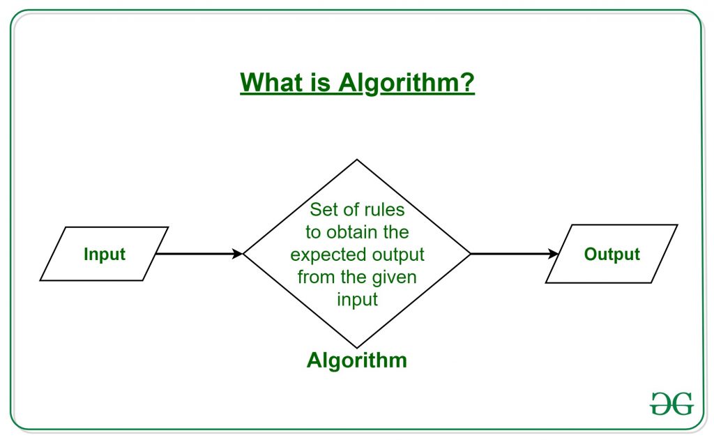
Use of the Algorithms:

Algorithms play a crucial role in various fields and have many applications. Some of the key areas where algorithms are used include:

• Computer Science: Algorithms form the basis of computer programming and are used to solve problems ranging from simple sorting and searching to complex tasks such as artificial intelligence and machine learning.
• Mathematics: Algorithms are used to solve mathematical problems, such as finding the optimal solution to a system of linear equations or finding the shortest path in a graph.
• Operations Research : Algorithms are used to optimize and make decisions in fields such as transportation, logistics, and resource allocation.
• Artificial Intelligence: Algorithms are the foundation of artificial intelligence and machine learning, and are used to develop intelligent systems that can perform tasks such as image recognition, natural language processing, and decision-making.
• Data Science: Algorithms are used to analyze, process, and extract insights from large amounts of data in fields such as marketing, finance, and healthcare.

These are just a few examples of the many applications of algorithms. The use of algorithms is continually expanding as new technologies and fields emerge, making it a vital component of modern society.

Algorithms can be simple and complex depending on what you want to achieve.

It can be understood by taking the example of cooking a new recipe. To cook a new recipe, one reads the instructions and steps and executes them one by one, in the given sequence. The result thus obtained is the new dish is cooked perfectly. Every time you use your phone, computer, laptop, or calculator you are using Algorithms. Similarly, algorithms help to do a task in programming to get the expected output.

The Algorithm designed are language-independent, i.e. they are just plain instructions that can be implemented in any language, and yet the output will be the same, as expected.

What is the need for algorithms?

• Algorithms are necessary for solving complex problems efficiently and effectively. 
• They help to automate processes and make them more reliable, faster, and easier to perform.
• Algorithms also enable computers to perform tasks that would be difficult or impossible for humans to do manually.
• They are used in various fields such as mathematics, computer science, engineering, finance, and many others to optimize processes, analyze data, make predictions, and provide solutions to problems.

What are the Characteristics of an Algorithm?

As one would not follow any written instructions to cook the recipe, but only the standard one. Similarly, not all written instructions for programming are an algorithm. For some instructions to be an algorithm, it must have the following characteristics:

• Clear and Unambiguous : The algorithm should be unambiguous. Each of its steps should be clear in all aspects and must lead to only one meaning.
• Well-Defined Inputs : If an algorithm says to take inputs, it should be well-defined inputs. It may or may not take input.
• Well-Defined Outputs: The algorithm must clearly define what output will be yielded and it should be well-defined as well. It should produce at least 1 output.
• Finite-ness: The algorithm must be finite, i.e. it should terminate after a finite time.
• Feasible: The algorithm must be simple, generic, and practical, such that it can be executed with the available resources. It must not contain some future technology or anything.
• Language Independent: The Algorithm designed must be language-independent, i.e. it must be just plain instructions that can be implemented in any language, and yet the output will be the same, as expected.
• Input : An algorithm has zero or more inputs. Each that contains a fundamental operator must accept zero or more inputs.
•   Output : An algorithm produces at least one output. Every instruction that contains a fundamental operator must accept zero or more inputs.
• Definiteness: All instructions in an algorithm must be unambiguous, precise, and easy to interpret. By referring to any of the instructions in an algorithm one can clearly understand what is to be done. Every fundamental operator in instruction must be defined without any ambiguity.
• Finiteness: An algorithm must terminate after a finite number of steps in all test cases. Every instruction which contains a fundamental operator must be terminated within a finite amount of time. Infinite loops or recursive functions without base conditions do not possess finiteness.
• Effectiveness: An algorithm must be developed by using very basic, simple, and feasible operations so that one can trace it out by using just paper and pencil.

Properties of Algorithm:

• It should terminate after a finite time.
• It should produce at least one output.
• It should take zero or more input.
• It should be deterministic means giving the same output for the same input case.
• Every step in the algorithm must be effective i.e. every step should do some work.

Types of Algorithms:

There are several types of algorithms available. Some important algorithms are:

1. Brute Force Algorithm :

It is the simplest approach to a problem. A brute force algorithm is the first approach that comes to finding when we see a problem.

2. Recursive Algorithm :

A recursive algorithm is based on recursion . In this case, a problem is broken into several sub-parts and called the same function again and again.

3. Backtracking Algorithm :

The backtracking algorithm builds the solution by searching among all possible solutions. Using this algorithm, we keep on building the solution following criteria. Whenever a solution fails we trace back to the failure point build on the next solution and continue this process till we find the solution or all possible solutions are looked after.

4. Searching Algorithm :

Searching algorithms are the ones that are used for searching elements or groups of elements from a particular data structure. They can be of different types based on their approach or the data structure in which the element should be found.

5. Sorting Algorithm :

Sorting is arranging a group of data in a particular manner according to the requirement. The algorithms which help in performing this function are called sorting algorithms. Generally sorting algorithms are used to sort groups of data in an increasing or decreasing manner.

6. Hashing Algorithm :

Hashing algorithms work similarly to the searching algorithm. But they contain an index with a key ID. In hashing, a key is assigned to specific data.

7. Divide and Conquer Algorithm :

This algorithm breaks a problem into sub-problems, solves a single sub-problem, and merges the solutions to get the final solution. It consists of the following three steps:

8. Greedy Algorithm :

In this type of algorithm, the solution is built part by part. The solution for the next part is built based on the immediate benefit of the next part. The one solution that gives the most benefit will be chosen as the solution for the next part.

9. Dynamic Programming Algorithm :

This algorithm uses the concept of using the already found solution to avoid repetitive calculation of the same part of the problem. It divides the problem into smaller overlapping subproblems and solves them.

10. Randomized Algorithm :

In the randomized algorithm, we use a random number so it gives immediate benefit. The random number helps in deciding the expected outcome.

To learn more about the types of algorithms refer to the article about “ Types of Algorithms “.

Advantages of Algorithms:

• It is easy to understand.
• An algorithm is a step-wise representation of a solution to a given problem.
• In an Algorithm the problem is broken down into smaller pieces or steps hence, it is easier for the programmer to convert it into an actual program.

Disadvantages of Algorithms :

• Writing an algorithm takes a long time so it is time-consuming.
• Understanding complex logic through algorithms can be very difficult.
• Branching and Looping statements are difficult to show in Algorithms (imp) .

How to Design an Algorithm?

To write an algorithm, the following things are needed as a pre-requisite: 

• The problem that is to be solved by this algorithm i.e. clear problem definition.
• The constraints of the problem must be considered while solving the problem.
• The input to be taken to solve the problem.
• The output is to be expected when the problem is solved.
• The solution to this problem is within the given constraints.

Then the algorithm is written with the help of the above parameters such that it solves the problem.

Example: Consider the example to add three numbers and print the sum.

Step 1: Fulfilling the pre-requisites  

• The problem that is to be solved by this algorithm : Add 3 numbers and print their sum.
• The constraints of the problem that must be considered while solving the problem : The numbers must contain only digits and no other characters.
• The input to be taken to solve the problem: The three numbers to be added.
• The output to be expected when the problem is solved: The sum of the three numbers taken as the input i.e. a single integer value.
• The solution to this problem, in the given constraints: The solution consists of adding the 3 numbers. It can be done with the help of the ‘+’ operator, or bit-wise, or any other method.

Step 2: Designing the algorithm

Now let’s design the algorithm with the help of the above pre-requisites:

• Declare 3 integer variables num1, num2, and num3.
• Take the three numbers, to be added, as inputs in variables num1, num2, and num3 respectively.
• Declare an integer variable sum to store the resultant sum of the 3 numbers.
• Add the 3 numbers and store the result in the variable sum.
• Print the value of the variable sum

Step 3: Testing the algorithm by implementing it.

To test the algorithm, let’s implement it in C language.

Here is the step-by-step algorithm of the code:

• Declare three variables num1, num2, and num3 to store the three numbers to be added.
• Declare a variable sum to store the sum of the three numbers.
• Use the cout statement to prompt the user to enter the first number.
• Use the cin statement to read the first number and store it in num1.
• Use the cout statement to prompt the user to enter the second number.
• Use the cin statement to read the second number and store it in num2.
• Use the cout statement to prompt the user to enter the third number.
• Use the cin statement to read and store the third number in num3.
• Calculate the sum of the three numbers using the + operator and store it in the sum variable.
• Use the cout statement to print the sum of the three numbers.
• The main function returns 0, which indicates the successful execution of the program.

Time complexity: O(1) Auxiliary Space: O(1) 

One problem, many solutions: The solution to an algorithm can be or cannot be more than one. It means that while implementing the algorithm, there can be more than one method to implement it. For example, in the above problem of adding 3 numbers, the sum can be calculated in many ways:

• Bit-wise operators

How to analyze an Algorithm? 

For a standard algorithm to be good, it must be efficient. Hence the efficiency of an algorithm must be checked and maintained. It can be in two stages:

1. Priori Analysis:

“Priori” means “before”. Hence Priori analysis means checking the algorithm before its implementation. In this, the algorithm is checked when it is written in the form of theoretical steps. This Efficiency of an algorithm is measured by assuming that all other factors, for example, processor speed, are constant and have no effect on the implementation. This is done usually by the algorithm designer. This analysis is independent of the type of hardware and language of the compiler. It gives the approximate answers for the complexity of the program.

2. Posterior Analysis:

“Posterior” means “after”. Hence Posterior analysis means checking the algorithm after its implementation. In this, the algorithm is checked by implementing it in any programming language and executing it. This analysis helps to get the actual and real analysis report about correctness(for every possible input/s if it shows/returns correct output or not), space required, time consumed, etc. That is, it is dependent on the language of the compiler and the type of hardware used.

What is Algorithm complexity and how to find it?

An algorithm is defined as complex based on the amount of Space and Time it consumes. Hence the Complexity of an algorithm refers to the measure of the time that it will need to execute and get the expected output, and the Space it will need to store all the data (input, temporary data, and output). Hence these two factors define the efficiency of an algorithm.  The two factors of Algorithm Complexity are:

• Time Factor : Time is measured by counting the number of key operations such as comparisons in the sorting algorithm.
• Space Factor : Space is measured by counting the maximum memory space required by the algorithm to run/execute.

Therefore the complexity of an algorithm can be divided into two types :

1. Space Complexity : The space complexity of an algorithm refers to the amount of memory required by the algorithm to store the variables and get the result. This can be for inputs, temporary operations, or outputs. 

How to calculate Space Complexity? The space complexity of an algorithm is calculated by determining the following 2 components:   

• Fixed Part: This refers to the space that is required by the algorithm. For example, input variables, output variables, program size, etc.
• Variable Part: This refers to the space that can be different based on the implementation of the algorithm. For example, temporary variables, dynamic memory allocation, recursion stack space, etc. Therefore Space complexity S(P) of any algorithm P is S(P) = C + SP(I) , where C is the fixed part and S(I) is the variable part of the algorithm, which depends on instance characteristic I.

Example: Consider the below algorithm for Linear Search

Step 1: START Step 2: Get n elements of the array in arr and the number to be searched in x Step 3: Start from the leftmost element of arr[] and one by one compare x with each element of arr[] Step 4: If x matches with an element, Print True. Step 5: If x doesn’t match with any of the elements, Print False. Step 6: END Here, There are 2 variables arr[], and x, where the arr[] is the variable part of n elements and x is the fixed part. Hence S(P) = 1+n. So, the space complexity depends on n(number of elements). Now, space depends on data types of given variables and constant types and it will be multiplied accordingly.

2. Time Complexity : The time complexity of an algorithm refers to the amount of time required by the algorithm to execute and get the result. This can be for normal operations, conditional if-else statements, loop statements, etc.

How to Calculate , Time Complexity? The time complexity of an algorithm is also calculated by determining the following 2 components: 

• Constant time part: Any instruction that is executed just once comes in this part. For example, input, output, if-else, switch, arithmetic operations, etc.

Example: In the algorithm of Linear Search above, the time complexity is calculated as follows:

Step 1: –Constant Time Step 2: — Variable Time (Taking n inputs) Step 3: –Variable Time (Till the length of the Array (n) or the index of the found element) Step 4: –Constant Time Step 5: –Constant Time Step 6: –Constant Time Hence, T(P) = 1 + n + n(1 + 1) + 1 = 2 + 3n, which can be said as T(n).

How to express an Algorithm?

• Natural Language:- Here we express the Algorithm in the natural English language. It is too hard to understand the algorithm from it.
• Flow Chart :- Here we express the Algorithm by making a graphical/pictorial representation of it. It is easier to understand than Natural Language.
• Pseudo Code :- Here we express the Algorithm in the form of annotations and informative text written in plain English which is very much similar to the real code but as it has no syntax like any of the programming languages, it can’t be compiled or interpreted by the computer. It is the best way to express an algorithm because it can be understood by even a layman with some school-level knowledge.

Please Login to comment...

Similar reads.

Improve your Coding Skills with Practice

What kind of Experience do you want to share?

• school Campus Bookshelves
• menu_book Bookshelves
• perm_media Learning Objects
• login Login
• how_to_reg Request Instructor Account
• hub Instructor Commons
• Download Page (PDF)
• Download Full Book (PDF)
• Periodic Table
• Physics Constants
• Scientific Calculator
• Reference & Cite
• Tools expand_more
• Readability

selected template will load here

This action is not available.

1: Algorithmic Problem Solving

• Last updated
• Save as PDF
• Page ID 46789

• Harrison Njoroge
• African Virtual University

Unit Objectives

Upon completion of this unit the learner should be able to:

• describe an algorithm
• explain the relationship between data and algorithm
• outline the characteristics of algorithms
• apply pseudo codes and flowcharts to represent algorithms

Unit Introduction

This unit introduces learners to data structures and algorithm course. The unit is on the different data structures and their algorithms that can help implement the different data structures in the computer. The application of the different data structures is presented by using examples of algorithms and which are not confined to a particular computer programming language.

• Data: the structural representation of logical relationships between elements of data
• Algorithm: finite sequence of steps for accomplishing some computational task
• Pseudo code: an informal high-level description of the operating principle of a computer program or other algorithm
• Flow chart: diagrammatic representation illustrates a solution model to a given problem.

Learning Activities

• 1.1: Activity 1 - Introduction to Algorithms and Problem Solving In this learning activity section, the learner will be introduced to algorithms and how to write algorithms to solve tasks faced by learners or everyday problems. Examples of the algorithm are also provided with a specific application to everyday problems that the learner is familiar with. The learners will particularly learn what is an algorithm, the process of developing a solution for a given task, and finally examples of application of the algorithms are given.
• 1.2: Activity 2 - The characteristics of an algorithm This section introduces the learners to the characteristics of algorithms. These characteristics make the learner become aware of what to ensure is basic, present and mandatory for any algorithm to qualify to be one. It also exposes the learner to what to expect from an algorithm to achieve or indicate. Key expectations are: the fact that an algorithm must be exact, terminate, effective, general among others.
• 1.3: Activity 3 - Using pseudo-codes and flowcharts to represent algorithms The student will learn how to design an algorithm using either a pseudo code or flowchart. Pseudo code is a mixture of English like statements, some mathematical notations and selected keywords from a programming language. It is one of the tools used to design and develop the solution to a task or problem. Pseudo codes have different ways of representing the same thing and emphasis is on the clarity and not style.
• 1.4: Unit Summary In this unit, you have seen what an algorithm is. Based on this knowledge, you should now be able to characterize an algorithm by stating its properties. We have explored the different ways of representing an algorithm such as using human language, pseudo codes and flow chart. You should now be able to present solutions to problems in form of an algorithm.

Forgot password? New user? Sign up

Existing user? Log in

Already have an account? Log in here.

• Pete Tomiello
• Debarghya Adhikari
• ANKIT JAVERI

An algorithm is a procedure that takes in input, follows a certain set of steps, and then produces an output. Oftentimes, the algorithm defines a desired relationship between the input and output. For example, if the problem that we are trying to solve is sorting a hand of cards, the problem might be defined as follows:

Problem : Sort the input. Input : A set of 5 cards. Output : The set of 5 input cards, sorted. Procedure : Up to the designer of the algorithm!

This last part is very important, it's the meat and substance of the algorithm. And, as an algorithm designer, you can do whatever you want to produce the desired output! Think about some ways you could sort 5 cards in your hand, and then click below to see some more ideas.

Algorithm Ideas

\(\hspace{0mm}\) We could simply toss them up in the air and pick them up again. Maybe they'll be sorted. If not, we can try it again and again until it works (spoiler: this is a bad algorithm). \(\hspace{0mm}\) We can sort them one at a time, left to right. Let's say our hand looks like {2, 4, 1, 9, 8}. Well, 2 and 4 are already sorted. But then we have a 1. That should go before 4, and it should go before 2. Now we have {1, 2, 4, 9, 8}. 9 is in the right spot because its higher than the card to its left, 4. But 8 is wrong because it's smaller than 9, so we'll just put it before 9. Now, we have {1, 2, 4, 8, 9}, and we're done. This is called insertion sort . \(\hspace{0mm}\) We can sort them two at a time, left to right. So, our hand is again {2, 4, 1, 9, 8}. 2 and 4 are good. 4 and 1 need to be swapped, so now we have {2, 1, 4, 9, 8}. 4 and 9 are good. 9 and 8 should be swapped, so now we have {2, 1, 4, 8, 9}. We have to start at the beginning again, but that's no problem. We look at the first pair and see that 2 and 1 need to switch, so now we have {1, 2, 4, 8, 9}, and we're done. This is called bubble sort . \(\hspace{0mm}\) There are a million ways to sort this hand of cards! Some are great, most are terrible. It's up to you as the algorithm designer to make a great one.

The study of algorithms involves finding the best ways to achieve the desired output given an input and a goal. Learning about algorithms is essential to being a successful computer programmer, and understanding them can help give you an idea of how computers work. So, if you'd like to learn to code, it's absolutely essential to learn about algorithms.

Algorithms and Computers

Properties of algorithms, types of algorithms, designing an algorithm, analyzing and evaluating an algorithm, hard algorithms.

Even though algorithms existed before the modern computer, they lie at the heart of computing and technology. Everything you've ever done on any piece of technology relies on algorithms because they tell technology what to do. Algorithms are responsible for your ability to surf the web at tolerable speeds. Imagine that you're visiting a website, and that website has a lot of unsorted content to show you. If it randomly picked a content order every time you visited it, and threw that order away and tried again if it wasn't correct, you'd be waiting for minutes, hours, or even days before your web page loaded!

Studying computer science and computer programming always involves algorithms because the study of algorithms teaches you to think like a machine so that you can program them in the best way possible. If you'd like to learn how to write applications, make websites, or do data analysis, you need to know about algorithms so that your code will run fast and run correctly.

On the theoretical side, many of the simpler algorithms have long since been discovered and heavily studied, but there are many areas left to research. For example, in theoretical computer science, a lingering question is whether P = NP , or in other words, "Are problems that can be quickly verified by a computer able to be quickly solved by a computer?" Currently, we don't think so. But if it turned out to be true, then computing and technology would experience an enormous speed increase that we would all benefit from. However, this would also mean that modern cryptography is not safe and any hacker could easily crack codes to any system in the world!

As computing grew, applications of computing grew along with it. In order to perform the algorithms that would enable those applications, computer scientists needed a way to represent and store that data. If we wanted to input a set of cards into a computer program, how would we store that data? How would we feed it into the algorithm? Early on, it was good enough to simply represent data as computer bits (zeroes and ones). However, that method could never last, it was too difficult and time-consuming.

Data structures were the answer. Their invention and research is paralleled by, and is often taught alongside, algorithms. The card sorting algorithm, for example, could take in an array of numbers to represent cards. More data structures were invented over time, and they allowed algorithm design to progress with them. With these in place, it became much easier to reason about, develop, and research algorithms.

Algorithms have 3 main properties that are important to remember during their design and analysis.

Algorithm Properties: Time complexity. This is the time an algorithm takes to complete, and it is often given using big O notation with its input as the independent variable. For example, if we want to search a card in the sorted \(n\) cards, we can do in logarithmic time, and the time complexity would be \(O\big(\log(n)\big)\). Space complexity. This is the space (in computer memory) the algorithm uses during its execution. Again, if we're sorting \(n\) cards, and we need to make an extra array of size \(n\) for each card to do so, the space complexity would be \(O\big(\log(n^2)\big)\). Correctness. An algorithm is correct if and only if, for every input, it halts and outputs the correct output. Contrary to what you might think, algorithms that are not correct are sometimes useful. For example, partially correct algorithms only guarantee that if the algorithm halts, the answer will be correct.

An algorithm can be expressed in a variety of ways, many of which you'll find in different wikis here on Brilliant.

A few examples of how an algorithm can be described are as follows: A high-level description . This might be in the form of text or prose that describes the algorithm: it's input, output, and goal. Generally, this does not involve implementation details of the algorithm. Formal definition . A formal definition will often give the input and output of the algorithm in formal mathematical terms. The procedure by which the output is achieved is also formally notated. This is a more mathematical way of representing an algorithm. Pseudo-code . This is a way of loosely formalizing an algorithm, and it is often used when learning algorithms. There are general implementation details; however, language-specific details are left out so as not to complicate things. Implementation . An implementation in a given language will be a piece of code that is understandable and runnable by a computer. It will fulfill the goals and procedure of the algorithm; however, it is harder to include high-level detail in an implementation because a computer will reject plain text.

There are many types of algorithms, and the language that describes them varies from textbook to textbook and from person to person. Some algorithm labels describe their function, and others describe the process by which they perform their function.

For example, there is a type of algorithm called string matching algorithms ; these algorithms find occurrences of an input string in larger strings or pieces of text. An example of a string matching algorithm is the Rabin-Karp algorithm , but there are many more. On the other hand, an example of a label that describes an algorithm's method for solving the problem is the divide and conquer algorithm . An example of this is binary search , which searches for a target in sorted input by cutting up the input into smaller pieces until the target is found.

A specific algorithm can span both classes. For example, a sorting algorithm that performs its sorting recursively could be described as either a sorting function or a recursive function.

Labels that describe function:

Labels that describe process:

When designing an algorithm, it is important to remember that computers are not infinitely fast and that computer memory is not infinitely large. That's why we make algorithms, after all. So, maybe you're designing an algorithm for a computer that is super fast but doesn't have much memory. Maybe you'll make some concessions on the computational requirements so that you can save memory.

But even if you never had to worry about speed or space, you still need to design a good algorithm. Why? You need to design a good algorithm because you need to know that the algorithm will do what you want it to do and that it will stop once it's done. You need to know that it will be correct.

The efficacy of the algorithm you're designing comes down to time complexity and space complexity . In an ideal world, the algorithm is efficient in both ways, but there is sometimes a tradeoff between them. It is up to the designer to weigh their needs appropriately in order to strike a balance.

It is also up to the designer to make a good algorithm. Doing so requires an understanding of algorithms as well as an understanding of existing algorithms to guide your design process. Otherwise, they might find themselves with a bad algorithm.

Two algorithms that do the same exact thing in different ways could have enormous differences in efficacy. In sorting, for example, bubble sort requires \(O(n)\) space during its execution. Quick sort , on the other hand, requires \(O\big(n\lg(n)\big)\) space. What does that mean for the programmer using those algorithms? Let's assume for simplicity that the input is just 1KB of data (or 8000 bits). Quicksort will require \(\lg(8000)\) times more space, or almost 13 times more space than bubble sort. Scale that up to inputs of 1GB or even 1TB, and this difference becomes very noticeable and very inefficient.

However, it's worth noting that quicksort runs faster than bubble sort by the same factor. Again, it's a tradeoff, and it's up to the designer to understand the tradeoffs and to optimize their design for their needs.

The analysis and evaluation of an algorithm is a two-step process. In the analysis portion, the algorithm is studied to learn about its properties: time/space complexity and correctness. Any method of describing the algorithm, as enumerated above , can be studied. However, that description must contain enough information about the inner workings of the algorithm to provide a clear picture of its procedure.

In general, there are a few ways to describe time complexity. There's the best-case , the average-case , and the worst-case for the algorithm. As a programmer, it's important to know each case so that you fully understand how your algorithm will operate. Which case you focus on is up to you, but the worst-case performance is often used as a benchmark for algorithms.

The evaluation portion is more qualitative and requires the observer to make decisions about the efficacy of the algorithm on its own, and as it relates to other similar algorithms. You might see the algorithm and notice that it is making some critical errors that increase its runtime. You might also discover that its runtime is drastically different than other algorithms that accomplish the same thing. In either case, the evaluation result is poor.

Let's take a look at the pseudo-code for an algorithm and try to analyze its time complexity. The following pseudo-code is that of insertion sort , a basic sorting algorithm. It takes as its input an array, \(A\), of the number and returns that same array, sorted. Note that this pseudo-code assumes 1-indexing (the first index in the array is 1, not 0).

1 2 3 4 5 6 7 8 Insertion_Sort(A) for j = 2 to j = A.length: current = A[j] i = j - 1 while i > 0 and A[i] > current: A[i+1] = A[i] i = i - 1 A[i + 1] = current Show Answer First, let's look at what this code is doing. We are given an input array of numbers, let's say [4, 2, 3, 7, 8] . The algorithm iterates through that array, starting with the second element, in this case, 2 . It calls this number current . It grabs the index right before current , which is 1 and whose value is 4 , and sets it equal to i . Now it wants to move 4 to the correct location. The while loop says "while the index i is more than 0, and while the number 2 is greater than its neighbor to the left, move 2 to the left and decrease i by 1". So, 2 is moved until it's in the correct spot with respect to the numbers seen so far by the algorithm. This pseudo-code can be analyzed by looking through this code line by line. In line 2, it has a for loop that iterates from the value 2 to the value A.length which is our input size, \(n.\) So, already we know for a fact that this algorithm is at least dependent linearly on our input size. In other words, the runtime of this algorithm is at least \(O(n)\) or \(\Omega(n)\). Everything inside the for loop must be executed \(n\) times, so we can ignore constant time operations such as lines 3, 4, and 8. Instead, line 5 is where the focus must shift because it is another iterable loop. The while loop on line 5 is similar to the for loop on line 2, but it has a variable number of times it can be repeated. That number can vary from 1 to \(n\) depending on how sorted our array is initially. If the input array is [2, 3, 4, 7, 8] , for example, the while loop will only run 1 time because each element is not greater than the element to its left. However, if the input is [8, 7, 4, 3, 2] , the while loop will need to run \(O(n)\) times. To see why, let's see what the array looks like after each iteration of the while loop: 1 2 3 4 5 0 (input). [8, 7, 4, 3, 2] 1: [7, 8, 4, 3, 2] 2: [4, 7, 8, 3, 2] 3: [3, 4, 7, 8, 2] 4: [2, 3, 4, 7, 8] See how between the \(3^\text{rd}\) and \(4^\text{th}\) iteration the 2 had to move all the way across the array? That's \(O(n)\) times. So, the for loop on line 2 iterates \(O(n)\) times. And the while loop on line 5 iterates anywhere from \(O(1)\) to \(O(n)\) times. So, the best-case runtime is \(O(n)\) when the input list is already sorted, and the worst-case is \(O(n^2)\) when it is sorted in reverse order. The average-case is a little trickier to understand. Basically, we'd expect any element in the input array to be less than half the elements to its left. Half of the elements is still \(\frac{n}{2},\) which is still \(O(n)\), so the average-case is also \(O(n^2)\).

The following pseudo-code represents an algorithm that takes as input an array of elements that can contain either positive integers or strings. In other words, the input could look like this [42, 'a', 1, 'hello', 3] .

The algorithm outputs an array with the following properties: elements in the output alternate between being a string and being an integer, and each element is less than or equal to the previous element of the same type (except for the elements at position 1 and 2, which are the largest of their respective types). In computer science, it is possible to sort strings ('b' > 'a', for example). This output will contain more elements than the input if the input does not have the same number of integers and strings.

What is the runtime of this algorithm?

For this example, assume that the sorting algorithm Reverse_Cheating_Sort(A) is a constant \(O(1)\) operation.

Typical algorithms are generally efficient. They run in polynomial time. In other words, their runtime can be defined as \(O(n^x)\) for some input \(n\) and some integer \(x\). However, there is a class of algorithms that do not currently have a polynomial-time solution. Some famous examples of this are the traveling salesperson problem or the set cover problem .

These problems are called NP-complete problems and are very interesting to study. Although no polynomial-time algorithm has ever been discovered for them, no one has proven that there can't be one out there, waiting to be discovered. Furthermore, if a solution was found for just one of them, a solution could be inferred for all of them!

There are currently various algorithms that make good approximations for solutions to these problems. They might use heuristics to cut down on runtime. However, the answer is not always exact, and the algorithm is therefore not correct.

The field of computer science contains many exciting areas to explore. In theory and algorithms, the question of NP-completeness and its relationship to other algorithms is one that has puzzled computer scientists for decades and that has many important implications for technology and for the world.

Problem Loading...

Note Loading...

Set Loading...

Learn Python practically and Get Certified .

Popular Tutorials

Popular examples, reference materials, learn python interactively, dsa introduction.

• What is an algorithm?
• Data Structure and Types
• Why learn DSA?
• Asymptotic Notations
• Master Theorem
• Divide and Conquer Algorithm

Data Structures (I)

• Types of Queue
• Circular Queue
• Priority Queue

Data Structures (II)

• Linked List
• Linked List Operations
• Types of Linked List
• Heap Data Structure
• Fibonacci Heap
• Decrease Key and Delete Node Operations on a Fibonacci Heap

Tree based DSA (I)

• Tree Data Structure
• Tree Traversal
• Binary Tree
• Full Binary Tree
• Perfect Binary Tree
• Complete Binary Tree
• Balanced Binary Tree
• Binary Search Tree

Tree based DSA (II)

• Insertion in a B-tree
• Deletion from a B-tree
• Insertion on a B+ Tree
• Deletion from a B+ Tree
• Red-Black Tree
• Red-Black Tree Insertion
• Red-Black Tree Deletion

Graph based DSA

• Graph Data Structure
• Spanning Tree
• Strongly Connected Components
• Adjacency Matrix
• Adjacency List
• DFS Algorithm
• Breadth-first Search

Bellman Ford's Algorithm

Sorting and Searching Algorithms

• Bubble Sort
• Selection Sort
• Insertion Sort
• Counting Sort
• Bucket Sort
• Linear Search
• Binary Search

Greedy Algorithms

Greedy Algorithm

• Ford-Fulkerson Algorithm
• Dijkstra's Algorithm
• Kruskal's Algorithm
• Prim's Algorithm
• Huffman Coding

Dynamic Programming

• Floyd-Warshall Algorithm
• Longest Common Sequence

Other Algorithms

• Backtracking Algorithm
• Rabin-Karp Algorithm

DSA Tutorials

Merge Sort Algorithm

• Selection Sort Algorithm

What is an Algorithm?

In computer programming terms, an algorithm is a set of well-defined instructions to solve a particular problem. It takes a set of input(s) and produces the desired output. For example,

An algorithm to add two numbers:

Take two number inputs

Add numbers using the + operator

Display the result

Qualities of a Good Algorithm

• Input and output should be defined precisely.
• Each step in the algorithm should be clear and unambiguous.
• Algorithms should be most effective among many different ways to solve a problem.
• An algorithm shouldn't include computer code. Instead, the algorithm should be written in such a way that it can be used in different programming languages.

Algorithm Examples

Algorithm to add two numbers

Algorithm to find the largest among three numbers

Algorithm to find all the roots of the quadratic equation

Algorithm to find the factorial

Algorithm to check prime number

Algorithm of Fibonacci series

Algorithm 1: Add two numbers entered by the user

Algorithm 2: find the largest number among three numbers, algorithm 3: find roots of a quadratic equation ax 2 + bx + c = 0, algorithm 4: find the factorial of a number, algorithm 5: check whether a number is prime or not, algorithm 6: find the fibonacci series till the term less than 1000, table of contents.

• Qualities of Good Algorithms
• Add Two Numbers
• Find Largest Number
• Roots of Quatratic Equation
• Find Factorial of a Number
• Check Prime Number
• Find Fibonacci Series

Sorry about that.

Related Tutorials

DS & Algorithms

Solve Me First Easy Problem Solving (Basic) Max Score: 1 Success Rate: 97.81%

Simple array sum easy problem solving (basic) max score: 10 success rate: 94.49%, compare the triplets easy problem solving (basic) max score: 10 success rate: 95.78%, a very big sum easy problem solving (basic) max score: 10 success rate: 98.81%, diagonal difference easy problem solving (basic) max score: 10 success rate: 95.99%, plus minus easy problem solving (basic) max score: 10 success rate: 98.38%, staircase easy problem solving (basic) max score: 10 success rate: 98.36%, mini-max sum easy problem solving (basic) max score: 10 success rate: 94.43%, birthday cake candles easy problem solving (basic) max score: 10 success rate: 97.12%, time conversion easy problem solving (basic) max score: 15 success rate: 92.30%, cookie support is required to access hackerrank.

Seems like cookies are disabled on this browser, please enable them to open this website

How to Solve an Algorithm Problem? | With Examples

If you’re stuck on an algorithm problem and not sure how to proceed, this blog post is for you! We’ll go over some general tips on solving algorithm problems, as well as a specific example of an algorithm .

Table of content:

Introduction.

• What are the 4 steps of algorithmic problem solving?
• Conclusion and References

What is an Algorithm?

What is an algorithm? Put simply, an algorithm is a step-by-step procedure for solving a problem. Algorithms can be written in any programming language, but they all share some common characteristics. First and foremost, algorithms are sequence tasks . That means that the steps in the algorithm must be done in order, and each step depends on the results of the previous steps. Secondly, algorithms are deterministic: given the same input data, exactly the same program will produce the same output every time. Finally, there are some measures for an algorithm to be efficient. Time and space: those two measures determine how efficient your algorithm is.

How to Solve an Algorithm Problem?

We’ll walk through some steps for solving a particular algorithm .

First, it’s important to know the basics of algorithms: every problem can be broken down into a sequence of steps that can be solved. This is known as the analysis of algorithms . Sketch out the basic structure of your algorithm on paper first or a board to avoid confusion. write some thoughts about which does what.

If a problem involves mathematical operations, conceptualizing it in terms of equations may be helpful. Break down the equation into its component parts and see if any of those particular pieces can be simplified or eliminated altogether. If so, that will lead to a solution for the whole equation.

Another strategy is to try reversing what initially seems like an impossible task. Algorithms problems often have stages were doing something one-way results in an error message or produces no useful output at all. Reverse engineer those steps and see if anything productive comes out.

What are the 4 steps of algorithmic problem-solving? and Example #1

Now that you know what an algorithm is, let’s jump into some examples and take a look at how these techniques can be put into practice…

In the following we will use the problem challenge from leetcode number #387 :

1) Understand the problem

The goal of any algorithm is to solve a problem.  When solving an algorithm problem, it is important to understand the problem and the steps involved in solving it. This understanding will allow you to correctly follow the instructions and complete the task. Answer the common questions to be sure that you really understand the problem. Questions like what it does and what kind of input I’m expecting. what kind of output I should receive? Are there some exceptions I should be aware of? etc…

The goal of this challenge is to write a function that takes in a string and returns the index of the first letter in the string that does not repeat. For example, if the string is “nerd”, the function should return 0, because the first letter “n” is the first non-repeating letter in the string. If the string is “abcdefg”, the function should return 0, because the first letter “a” is the first non-repeating letter in the string.

If the string does not contain any non-repeating letters, the function should return -1. For example, if the input string is “abcabc”, the function should return -1, because no letter in the string is unique or non-repeating.

2) Break the problem down

When solving algorithms problems , breaking them down into smaller parts is usually the best way to go. Once you understand how each part works and interacts with the others, you can solve the problem more quickly.

To solve this challenge, we need to do the following:

• Iterate over the letters in the input string, and for each letter, keep track of how many times it appears in the string. We can do this using an object, dictionary, or map, where the keys are the letters in the string, and the values are the counts for each letter.
• Once we have counted the occurrences of each letter in the string, we need to find the index of the first letter that has a count of 1 (i.e. the first non-repeating letter). To do this, we can iterate over the letters in the string again, and for each letter, check if its count in the object/dictionary is 1. If it is, we return the index of the letter.
• If we reach the end of the loop without finding any value that has only 1 or non-repeating letters, we return -1 to indicate that no non-repeating letters were found.

3) Find your solution

We found one solution and the key steps in this solution are to keep track of the counts of each letter in the input string, and then to search for the first letter with a count of 1.  If the count of this letter is 1 meaning that this letter only shows one time in the string. These steps can be implemented in a variety of ways, depending on the language and tools you are using to solve the challenge.

We will be demonstrating the solution with two programming languages JavaScript and Python:

The source code in JavaScript:

Here are some examples of how this function can be used:

The source code in Python :

4) Check your solution

Checking your solution again answers some questions like can I write a better code? by better I mean is the code I provided covering all cases of inputs? is it efficient? and by efficient, I mean using fewer computer resources when possible. If you’re comfortable with your answers then check if there is another solution out there for the same problem you solved, if any are found. go through them I learned a lot by doing that. Also get some feedback on your code, that way you’ll learn many ways of approaching a problem to solve it.

As we mentioned above we asked ourselves these questions but the algorithm we wrote couldn’t go through all the different cases successfully: for example, The code can’t handle the case when we handled two cases of the same character “L” and “l” in the word “Level”

So we need to address that in the following:

Now let’s revisit the code that we wrote up and see if we can come up with another solution that will cover the all different cases of a character.

The source code in JavaScript :

Now that you learned from the first example, let’s jump into another challenge and apply the same techniques we used above:

This example from leetcode problem #125 Valid Palindrome

Learn as much information as you can about the problem what is a Palindrome? Ask yourself what input you expect and what output is expected.

The Palindrome is a word, phrase, or sentence that is spelled backward as forwards. We expect a string and we can do a function that first cleans that string from any non-alphanumeric, then reverses it and compares it with the original string.

Here is a step-by-step explanation of the algorithm in plain English:

• Convert all uppercase letters in the string to lowercase. This is done so that the case of the letters in the string does not affect the outcome of the comparison.
• Remove all non-alphanumeric characters from the string. This is done because only alphanumeric characters are relevant for determining if a string is a palindrome.
• Reverse the resulting string. This is done so that we can compare the reversed string with the original string.
• Compare the reversed string with the original string. If they are the same, then the original string is a palindrome. Otherwise, it is not.

Here is an example of how this algorithm would work on the string “A man, a plan, a canal: Panama”:

• The string is converted to lowercase, so it becomes “a man, a plan, a canal: panama”.
• All non-alphanumeric characters are removed, so the string becomes “amanaplanacanalpanama”.
• The string is reversed, so it becomes “amanaplanacanalpanama”.
• The reversed string is compared with the original string, and since they are the same, the function returns true, indicating that the original string is a palindrome.

According to the steps we wrote in the previous stage, let’s put them into action and code it up.

The source code in Python:

We can make it more efficient by using the pointers method let’s break it down into a few points below:

• Create left and right pointers (will be represented by indices)
• Make each pointer move to the middle direction
• While moving to check each letter for both pointers are the same

Conclusion and references

There are many resources available to help you out, and with more practice , you’ll be able to solve many algorithm problems that come your way . This video is one of the great resources to learn about algorithms and data structures from FreeCodeCamp

It is important to keep a cool head and not get bogged down in frustration. Algorithms problems can be difficult, but with patience and perseverance, they can be solved.

When you are solving an algorithm problem, it is important to be able to check your solution against other solutions if possible to see how others approach the same problem. This is will help you to retain and understand the logic behind the different solutions so you’ll need this kind of knowledge in the future solving problems.

By following the steps outlined in this article, you will be able to solve algorithm problems with ease. Remember to keep a notebook or excel sheet with all of your solutions so that you can revisit them later on that way you will gain maximum retention of the logic.

If you want to learn more about algorithms and programming , sign up for our mailing list. We’ll send you tips, tricks, and resources to help you improve your skills.

Ahmed Radwan

Reach out if you want to join me and write articles with the nerds 🙂

How to Make Your Corporate Website Stand Out With These 10 Tips

How to write clean code and best practices, you may also like, top 100 problems on leetcode and its solutions – part1, learn essential javascript methods and objects, react: what is the one-way data flow and jsx rules.

• Smart Devices
• Programming
• Web Development
• Presentation
• Infographics

• Bipolar Disorder
• Therapy Center
• When To See a Therapist
• Types of Therapy
• Best Online Therapy
• Best Couples Therapy
• Best Family Therapy
• Managing Stress
• Sleep and Dreaming
• Understanding Emotions
• Self-Improvement
• Healthy Relationships
• Student Resources
• Personality Types
• Guided Meditations
• Verywell Mind Insights
• 2023 Verywell Mind 25
• Mental Health in the Classroom
• Editorial Process
• Meet Our Review Board
• Crisis Support

Overview of the Problem-Solving Mental Process

Kendra Cherry, MS, is a psychosocial rehabilitation specialist, psychology educator, and author of the "Everything Psychology Book."

Rachel Goldman, PhD FTOS, is a licensed psychologist, clinical assistant professor, speaker, wellness expert specializing in eating behaviors, stress management, and health behavior change.

• Identify the Problem
• Define the Problem
• Form a Strategy
• Organize Information
• Allocate Resources
• Monitor Progress
• Evaluate the Results

Frequently Asked Questions

Problem-solving is a mental process that involves discovering, analyzing, and solving problems. The ultimate goal of problem-solving is to overcome obstacles and find a solution that best resolves the issue.

The best strategy for solving a problem depends largely on the unique situation. In some cases, people are better off learning everything they can about the issue and then using factual knowledge to come up with a solution. In other instances, creativity and insight are the best options.

It is not necessary to follow problem-solving steps sequentially, It is common to skip steps or even go back through steps multiple times until the desired solution is reached.

In order to correctly solve a problem, it is often important to follow a series of steps. Researchers sometimes refer to this as the problem-solving cycle. While this cycle is portrayed sequentially, people rarely follow a rigid series of steps to find a solution.

The following steps include developing strategies and organizing knowledge.

1. Identifying the Problem

While it may seem like an obvious step, identifying the problem is not always as simple as it sounds. In some cases, people might mistakenly identify the wrong source of a problem, which will make attempts to solve it inefficient or even useless.

Some strategies that you might use to figure out the source of a problem include :

• Asking questions about the problem
• Breaking the problem down into smaller pieces
• Looking at the problem from different perspectives
• Conducting research to figure out what relationships exist between different variables

2. Defining the Problem

After the problem has been identified, it is important to fully define the problem so that it can be solved. You can define a problem by operationally defining each aspect of the problem and setting goals for what aspects of the problem you will address

At this point, you should focus on figuring out which aspects of the problems are facts and which are opinions. State the problem clearly and identify the scope of the solution.

3. Forming a Strategy

After the problem has been identified, it is time to start brainstorming potential solutions. This step usually involves generating as many ideas as possible without judging their quality. Once several possibilities have been generated, they can be evaluated and narrowed down.

The next step is to develop a strategy to solve the problem. The approach used will vary depending upon the situation and the individual's unique preferences. Common problem-solving strategies include heuristics and algorithms.

• Heuristics are mental shortcuts that are often based on solutions that have worked in the past. They can work well if the problem is similar to something you have encountered before and are often the best choice if you need a fast solution.
• Algorithms are step-by-step strategies that are guaranteed to produce a correct result. While this approach is great for accuracy, it can also consume time and resources.

Heuristics are often best used when time is of the essence, while algorithms are a better choice when a decision needs to be as accurate as possible.

4. Organizing Information

Before coming up with a solution, you need to first organize the available information. What do you know about the problem? What do you not know? The more information that is available the better prepared you will be to come up with an accurate solution.

When approaching a problem, it is important to make sure that you have all the data you need. Making a decision without adequate information can lead to biased or inaccurate results.

5. Allocating Resources

Of course, we don't always have unlimited money, time, and other resources to solve a problem. Before you begin to solve a problem, you need to determine how high priority it is.

If it is an important problem, it is probably worth allocating more resources to solving it. If, however, it is a fairly unimportant problem, then you do not want to spend too much of your available resources on coming up with a solution.

At this stage, it is important to consider all of the factors that might affect the problem at hand. This includes looking at the available resources, deadlines that need to be met, and any possible risks involved in each solution. After careful evaluation, a decision can be made about which solution to pursue.

6. Monitoring Progress

After selecting a problem-solving strategy, it is time to put the plan into action and see if it works. This step might involve trying out different solutions to see which one is the most effective.

It is also important to monitor the situation after implementing a solution to ensure that the problem has been solved and that no new problems have arisen as a result of the proposed solution.

Effective problem-solvers tend to monitor their progress as they work towards a solution. If they are not making good progress toward reaching their goal, they will reevaluate their approach or look for new strategies .

7. Evaluating the Results

After a solution has been reached, it is important to evaluate the results to determine if it is the best possible solution to the problem. This evaluation might be immediate, such as checking the results of a math problem to ensure the answer is correct, or it can be delayed, such as evaluating the success of a therapy program after several months of treatment.

Once a problem has been solved, it is important to take some time to reflect on the process that was used and evaluate the results. This will help you to improve your problem-solving skills and become more efficient at solving future problems.

A Word From Verywell​

It is important to remember that there are many different problem-solving processes with different steps, and this is just one example. Problem-solving in real-world situations requires a great deal of resourcefulness, flexibility, resilience, and continuous interaction with the environment.

Get Advice From The Verywell Mind Podcast

Hosted by therapist Amy Morin, LCSW, this episode of The Verywell Mind Podcast shares how you can stop dwelling in a negative mindset.

Follow Now : Apple Podcasts / Spotify / Google Podcasts

You can become a better problem solving by:

• Practicing brainstorming and coming up with multiple potential solutions to problems
• Being open-minded and considering all possible options before making a decision
• Breaking down problems into smaller, more manageable pieces
• Asking for help when needed
• Researching different problem-solving techniques and trying out new ones
• Learning from mistakes and using them as opportunities to grow

It's important to communicate openly and honestly with your partner about what's going on. Try to see things from their perspective as well as your own. Work together to find a resolution that works for both of you. Be willing to compromise and accept that there may not be a perfect solution.

Take breaks if things are getting too heated, and come back to the problem when you feel calm and collected. Don't try to fix every problem on your own—consider asking a therapist or counselor for help and insight.

If you've tried everything and there doesn't seem to be a way to fix the problem, you may have to learn to accept it. This can be difficult, but try to focus on the positive aspects of your life and remember that every situation is temporary. Don't dwell on what's going wrong—instead, think about what's going right. Find support by talking to friends or family. Seek professional help if you're having trouble coping.

Davidson JE, Sternberg RJ, editors.  The Psychology of Problem Solving .  Cambridge University Press; 2003. doi:10.1017/CBO9780511615771

Sarathy V. Real world problem-solving .  Front Hum Neurosci . 2018;12:261. Published 2018 Jun 26. doi:10.3389/fnhum.2018.00261

By Kendra Cherry, MSEd Kendra Cherry, MS, is a psychosocial rehabilitation specialist, psychology educator, and author of the "Everything Psychology Book."

Algorithm in Math – Definition with Examples

What is an algorithm, advantages of algorithms, properties of algorithms, solved examples, practice problems, frequently asked questions.

An algorithm is a step-by-step process to solve a particular problem.

Think of it as a mathematical “recipe” to get to the bottom of a problem. If you follow the steps, you’ll be able to get to the answer in no time!

Example of an algorithm:  A simple example of an algorithm you use every day is your morning routine. Say you get up at 6:30 a.m. to go to school. If you always get up, brush your teeth, drink water, go to the bathroom, and then have a bath, that can be the algorithm your body follows! Algorithms are all around us. It’s important to spot them to know how they function and later create our own.

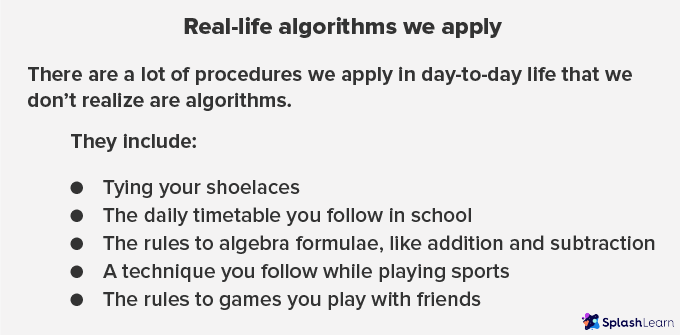
There are a lot of procedures we apply in day-to-day life that we don’t realize are algorithms.

They include:

Tying your shoelaces

The daily timetable you follow in school

The rules to algebra formulae, like addition and subtraction

A technique you follow while playing sports

The rules to games you play with friends

Algorithms in Math

Definition of Math Algorithm An algorithm in math is a procedure, a description of a set of steps that can be used to solve a mathematical computation. For example, a step-by-step procedure used in long divisions is a common example of a mathematical algorithm.

Example of Math Algorithm:  The process of solving a mathematical problem such as, “What is 82 divided by 3?” could be achieved by doing the following algorithm:

How many times does 3 go into 8?

The answer is 2.

How many are left over now? 2

Put the 2 (tens) in front of the 3.

How many times does 3 go into 22?

The answer is 7, with a remainder of one.

And of course, the answer is 27 with a remainder of 1.

Standard Algorithm for Addition 

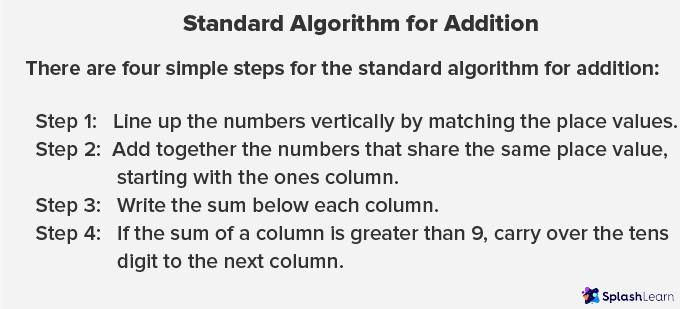
There are four simple steps for the standard algorithm for addition:

Step 1: Line up the numbers vertically by matching the place values.

Step 2: Add together the numbers that share the same place value, starting with the ones column.

Step 3: Write the sum below each column.

Step 4: If the sum of a column is greater than 9, carry over the tens digit to the next column.

Standard Algorithm for Subtraction 

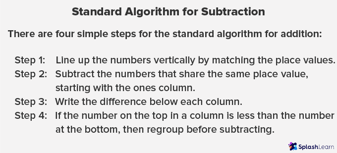
Step 2: Subtract the numbers that share the same place value, starting with the ones column.

Step 3: Write the difference below each column.

Step 4: If the number on the top in a column is less than the number at the bottom, then regroup before subtracting.

Standard Algorithm for Multiplication

Follow the link  to check the standard algorithm of multiplication. 

Related Worksheets

Algorithms are essential because of the large variety of applications in which they are used. Understanding how algorithms work is also crucial for developing problem-solving skills and building logical reasoning. Listed below are a few advantages of an algorithm:

• The algorithm creation process allows you to look at something in a rational and calculative manner, which helps greatly when it comes to solving different kinds of problems.
• Algorithms aid in bridging the communication gap, where following the procedure will help you reach the solution needed without going over the process repeatedly. You can follow the rules set up beforehand to reach the solution quicker.
• Algorithms use a definite procedure, and by using and optimizing them, people can solve problems much quicker. 
• Algorithms are easy to debug because each step has its logical sequence.
• When we use algorithms, we can break down the problems into smaller steps or pieces, and therefore a programmer can easily convert them into an actual program.

Once you understand the foundation of algorithms, you will be able to create your own, saving yourself a lot of time. With SplashLearn’s fun activities and games, you can put your mathematical skills to the test and find algorithms in the questions you solve.

Algorithms should be used to solve three objectives:

• Correctly execute a task:  The job you want to do should be carried out with the intended results.
• Efficiently process the information given:  Your system’s time and resources should be appropriately used to understand and later resolve the problem.
• Be easily understood:  Algorithms are meant to make a job easier and, ideally, should be kept at a fundamental level of understanding.

Examples of algorithms in the real world

Many companies in the real world use algorithms to help their customers or grow their businesses and often try to improve those every day.

• YouTube : When you watch a few videos of a certain channel, you’ll notice that more and more videos by the same channel get recommended to you. It is due to YouTube’s recommendation algorithm, which collects information from your previous history to present videos of the same kind in your feed, so that you continue to watch videos on the platform.
• Social media : If you navigate to the ‘Explore’ page on Instagram, you’ll notice that many of the posts that show up are related to the ones you usually search for or like/comment on. The algorithm here identifies the posts you interact with and shows you more such posts because it believes that you enjoy such posts.
• Google : Google uses a very famous algorithm called PageRank to sort search results into an order that shows the most visited and authentic sites at the top. This algorithm considers dozens of parameters and provides the websites you would like to find fast.
• Lyft/Uber : Cab sharing companies like Lyft or Uber use positioning algorithms to help customers find vehicles close to them for an optimal experience. These global positioning algorithms also help drivers find the fastest routes to reach a certain destination. Algorithms also help such applications decide which customer they should pick or drop first.
• Facial recognition : Whenever companies require users to be verified, they can move past methods like user IDs and passwords to more secure authentications like facial recognition. Here, algorithms are used to identify a person and check if they have access to the things they want to get to.

Tips to Master Algorithms

You can master algorithms by learning how to spot them in your day-to-day life. After that, you can break down the algorithm into bite-sized steps. You might have to test it a few times to notice a pattern in the way something takes place, but once you find it, you’ll be able to spot it again and again.

Try to figure out why each step in a process takes place. Once you understand why something happens, you’ll be able to connect the dots easier and figure out the logical sequence of events. In addition, it comes in very handy for figuring out how to create algorithms for yourself. With the help of the fun activities and games on SplashLearn, you’ll be able to master the basics of algorithms in no time!

Example 1 : Write down the steps for making peanut butter and jelly sandwich.

Answer:  Steps for making a peanut butter and jelly sandwich: Step 1: Take 2 slices of bread. Step 2: Apply peanut butter on one side of a slice. Step 3: Apply jelly on one side of the other slice. Step 4: Press both the slices of bread together.

Example 2:  Write down the steps for the standard algorithm of subtraction.

Answer:  The standard algorithm for subtraction follows these 4 steps: Step 1: Line up the numbers vertically by matching the place values. Step 2: Subtract the numbers that share the same place value, starting with the ones column. Step 3: Write the difference below each column. Step 4: If the number on the top in a column is less than the number at the bottom, then regroup before subtracting.

Example 3:  Write an algorithm to know whether a number is odd or even.

Answer:  The algorithm to find whether a number is odd or even: Step 1: Divide the number by 2. Step 2: If the number is completely divisible by 2, it is even, else it is odd.

Example 4:  Write an algorithm to find the area of a rectangle.

Answer:  The algorithm to find the area of the rectangle: Step 1: Record the length of the shorter side as ‘b’. Step 2: Record the length of the longer side as ‘l’. Step 3: Area of a rectangle will be the product of ‘l’ and ‘b’.

Attend this Quiz & Test your knowledge.

Which sequence will give the correct picture of an owl?

Which sequence will give the correct algorithm for boiling water? 1. Heat the pot until water boils 2. Turn the stove on 3. Take an empty pot 4. Put the water-filled pot on the fire 5. Pour water in empty pot

What will be the first step of addition algorithm, which of the following correctly multiplies 45 ✕ 7 using the standard algorithm.

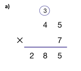
How are algorithms related to math?

An algorithm in mathematics is a procedure, a set of steps describing how a mathematical problem can be solved. For example, the step by step procedures of long division or decimal multiplication.

Where do we use algorithms in real life?

Algorithms are primarily used in computing. In our day-to-day lives, algorithms can be seen all around us, solving our daily problems. YouTube and Netflix recommendations, Google searches, GPS applications, among others, all are powered by algorithms.

What are the disadvantages of using algorithms?

Algorithms are hard to apply to bigger and more complex tasks. They are time-consuming. It is not always easy to show branching and looping in algorithms. It can be very challenging to understand complex logic applied in algorithms.

What are the important characteristics of algorithms?

The steps of algorithms should be precisely stated. The algorithm receives input and produces an output after executing a finite number of instructions.

RELATED POSTS

• Meters to Feet (m to ft) Conversion – Table, Formula, Method
• Angles of Parallelogram – Definition, Properties, Theorems, Examples
• Stack – Definition with Examples
• Linear Equations – Definition, Graph, Examples, Facts, FAQs
• Volume of Cuboid – Definition, Formula, Derivation, Examples, FAQs

Math & ELA | PreK To Grade 5

Kids see fun., you see real learning outcomes..

Make study-time fun with 14,000+ games & activities, 450+ lesson plans, and more—free forever.

Parents, Try for Free Teachers, Use for Free

Thank you for visiting nature.com. You are using a browser version with limited support for CSS. To obtain the best experience, we recommend you use a more up to date browser (or turn off compatibility mode in Internet Explorer). In the meantime, to ensure continued support, we are displaying the site without styles and JavaScript.

• View all journals
• My Account Login
• Explore content
• About the journal
• Publish with us
• Sign up for alerts
• Open access
• Published: 10 April 2024

A hybrid particle swarm optimization algorithm for solving engineering problem

• Jinwei Qiao 1 , 2 ,
• Guangyuan Wang 1 , 2 ,
• Zhi Yang 1 , 2 ,
• Xiaochuan Luo 3 ,
• Jun Chen 1 , 2 ,
• Kan Li 4 &
• Pengbo Liu 1 , 2  

Scientific Reports volume  14 , Article number:  8357 ( 2024 ) Cite this article

375 Accesses

Metrics details

• Computational science
• Mechanical engineering

To overcome the disadvantages of premature convergence and easy trapping into local optimum solutions, this paper proposes an improved particle swarm optimization algorithm (named NDWPSO algorithm) based on multiple hybrid strategies. Firstly, the elite opposition-based learning method is utilized to initialize the particle position matrix. Secondly, the dynamic inertial weight parameters are given to improve the global search speed in the early iterative phase. Thirdly, a new local optimal jump-out strategy is proposed to overcome the "premature" problem. Finally, the algorithm applies the spiral shrinkage search strategy from the whale optimization algorithm (WOA) and the Differential Evolution (DE) mutation strategy in the later iteration to accelerate the convergence speed. The NDWPSO is further compared with other 8 well-known nature-inspired algorithms (3 PSO variants and 5 other intelligent algorithms) on 23 benchmark test functions and three practical engineering problems. Simulation results prove that the NDWPSO algorithm obtains better results for all 49 sets of data than the other 3 PSO variants. Compared with 5 other intelligent algorithms, the NDWPSO obtains 69.2%, 84.6%, and 84.6% of the best results for the benchmark function ( \({f}_{1}-{f}_{13}\) ) with 3 kinds of dimensional spaces (Dim = 30,50,100) and 80% of the best optimal solutions for 10 fixed-multimodal benchmark functions. Also, the best design solutions are obtained by NDWPSO for all 3 classical practical engineering problems.

Similar content being viewed by others

Neural operators for accelerating scientific simulations and design

Kamyar Azizzadenesheli, Nikola Kovachki, … Anima Anandkumar

Spike sorting with Kilosort4

Marius Pachitariu, Shashwat Sridhar, … Carsen Stringer

Physics-informed machine learning

George Em Karniadakis, Ioannis G. Kevrekidis, … Liu Yang

Introduction

In the ever-changing society, new optimization problems arise every moment, and they are distributed in various fields, such as automation control 1 , statistical physics 2 , security prevention and temperature prediction 3 , artificial intelligence 4 , and telecommunication technology 5 . Faced with a constant stream of practical engineering optimization problems, traditional solution methods gradually lose their efficiency and convenience, making it more and more expensive to solve the problems. Therefore, researchers have developed many metaheuristic algorithms and successfully applied them to the solution of optimization problems. Among them, Particle swarm optimization (PSO) algorithm 6 is one of the most widely used swarm intelligence algorithms.

However, the basic PSO has a simple operating principle and solves problems with high efficiency and good computational performance, but it suffers from the disadvantages of easily trapping in local optima and premature convergence. To improve the overall performance of the particle swarm algorithm, an improved particle swarm optimization algorithm is proposed by the multiple hybrid strategy in this paper. The improved PSO incorporates the search ideas of other intelligent algorithms (DE, WOA), so the improved algorithm proposed in this paper is named NDWPSO. The main improvement schemes are divided into the following 4 points: Firstly, a strategy of elite opposition-based learning is introduced into the particle population position initialization. A high-quality initialization matrix of population position can improve the convergence speed of the algorithm. Secondly, a dynamic weight methodology is adopted for the acceleration coefficients by combining the iterative map and linearly transformed method. This method utilizes the chaotic nature of the mapping function, the fast convergence capability of the dynamic weighting scheme, and the time-varying property of the acceleration coefficients. Thus, the global search and local search of the algorithm are balanced and the global search speed of the population is improved. Thirdly, a determination mechanism is set up to detect whether the algorithm falls into a local optimum. When the algorithm is “premature”, the population resets 40% of the position information to overcome the local optimum. Finally, the spiral shrinking mechanism combined with the DE/best/2 position mutation is used in the later iteration, which further improves the solution accuracy.

The structure of the paper is given as follows: Sect. “ Particle swarm optimization (PSO) ” describes the principle of the particle swarm algorithm. Section “ Improved particle swarm optimization algorithm ” shows the detailed improvement strategy and a comparison experiment of inertia weight is set up for the proposed NDWPSO. Section “ Experiment and discussion ” includes the experimental and result discussion sections on the performance of the improved algorithm. Section “ Conclusions and future works ” summarizes the main findings of this study.

Literature review

This section reviews some metaheuristic algorithms and other improved PSO algorithms. A simple discussion about recently proposed research studies is given.

Metaheuristic algorithms

A series of metaheuristic algorithms have been proposed in recent years by using various innovative approaches. For instance, Lin et al. 7 proposed a novel artificial bee colony algorithm (ABCLGII) in 2018 and compared ABCLGII with other outstanding ABC variants on 52 frequently used test functions. Abed-alguni et al. 8 proposed an exploratory cuckoo search (ECS) algorithm in 2021 and carried out several experiments to investigate the performance of ECS by 14 benchmark functions. Brajević 9 presented a novel shuffle-based artificial bee colony (SB-ABC) algorithm for solving integer programming and minimax problems in 2021. The experiments are tested on 7 integer programming problems and 10 minimax problems. In 2022, Khan et al. 10 proposed a non-deterministic meta-heuristic algorithm called Non-linear Activated Beetle Antennae Search (NABAS) for a non-convex tax-aware portfolio selection problem. Brajević et al. 11 proposed a hybridization of the sine cosine algorithm (HSCA) in 2022 to solve 15 complex structural and mechanical engineering design optimization problems. Abed-Alguni et al. 12 proposed an improved Salp Swarm Algorithm (ISSA) in 2022 for single-objective continuous optimization problems. A set of 14 standard benchmark functions was used to evaluate the performance of ISSA. In 2023, Nadimi et al. 13 proposed a binary starling murmuration optimization (BSMO) to select the effective features from different important diseases. In the same year, Nadimi et al. 14 systematically reviewed the last 5 years' developments of WOA and made a critical analysis of those WOA variants. In 2024, Fatahi et al. 15 proposed an Improved Binary Quantum-based Avian Navigation Optimizer Algorithm (IBQANA) for the Feature Subset Selection problem in the medical area. Experimental evaluation on 12 medical datasets demonstrates that IBQANA outperforms 7 established algorithms. Abed-alguni et al. 16 proposed an Improved Binary DJaya Algorithm (IBJA) to solve the Feature Selection problem in 2024. The IBJA’s performance was compared against 4 ML classifiers and 10 efficient optimization algorithms.

Improved PSO algorithms

Many researchers have constantly proposed some improved PSO algorithms to solve engineering problems in different fields. For instance, Yeh 17 proposed an improved particle swarm algorithm, which combines a new self-boundary search and a bivariate update mechanism, to solve the reliability redundancy allocation problem (RRAP) problem. Solomon et al. 18 designed a collaborative multi-group particle swarm algorithm with high parallelism that was used to test the adaptability of Graphics Processing Units (GPUs) in distributed computing environments. Mukhopadhyay and Banerjee 19 proposed a chaotic multi-group particle swarm optimization (CMS-PSO) to estimate the unknown parameters of an autonomous chaotic laser system. Duan et al. 20 designed an improved particle swarm algorithm with nonlinear adjustment of inertia weights to improve the coupling accuracy between laser diodes and single-mode fibers. Sun et al. 21 proposed a particle swarm optimization algorithm combined with non-Gaussian stochastic distribution for the optimal design of wind turbine blades. Based on a multiple swarm scheme, Liu et al. 22 proposed an improved particle swarm optimization algorithm to predict the temperatures of steel billets for the reheating furnace. In 2022, Gad 23 analyzed the existing 2140 papers on Swarm Intelligence between 2017 and 2019 and pointed out that the PSO algorithm still needs further research. In general, the improved methods can be classified into four categories:

Adjusting the distribution of algorithm parameters. Feng et al. 24 used a nonlinear adaptive method on inertia weights to balance local and global search and introduced asynchronously varying acceleration coefficients.

Changing the updating formula of the particle swarm position. Both papers 25 and 26 used chaotic mapping functions to update the inertia weight parameters and combined them with a dynamic weighting strategy to update the particle swarm positions. This improved approach enables the particle swarm algorithm to be equipped with fast convergence of performance.

The initialization of the swarm. Alsaidy and Abbood proposed 27 a hybrid task scheduling algorithm that replaced the random initialization of the meta-heuristic algorithm with the heuristic algorithms MCT-PSO and LJFP-PSO.

Combining with other intelligent algorithms: Liu et al. 28 introduced the differential evolution (DE) algorithm into PSO to increase the particle swarm as diversity and reduce the probability of the population falling into local optimum.

Particle swarm optimization (PSO)

The particle swarm optimization algorithm is a population intelligence algorithm for solving continuous and discrete optimization problems. It originated from the social behavior of individuals in bird and fish flocks 6 . The core of the PSO algorithm is that an individual particle identifies potential solutions by flight in a defined constraint space adjusts its exploration direction to approach the global optimal solution based on the shared information among the group, and finally solves the optimization problem. Each particle \(i\) includes two attributes: velocity vector \({V}_{i}=\left[{v}_{i1},{v}_{i2},{v}_{i3},{...,v}_{ij},{...,v}_{iD},\right]\) and position vector \({X}_{i}=[{x}_{i1},{x}_{i2},{x}_{i3},...,{x}_{ij},...,{x}_{iD}]\) . The velocity vector is used to modify the motion path of the swarm; the position vector represents a potential solution for the optimization problem. Here, \(j=\mathrm{1,2},\dots ,D\) , \(D\) represents the dimension of the constraint space. The equations for updating the velocity and position of the particle swarm are shown in Eqs. ( 1 ) and ( 2 ).

Here \({Pbest}_{i}^{k}\) represents the previous optimal position of the particle \(i\) , and \({Gbest}\) is the optimal position discovered by the whole population. \(i=\mathrm{1,2},\dots ,n\) , \(n\) denotes the size of the particle swarm. \({c}_{1}\) and \({c}_{2}\) are the acceleration constants, which are used to adjust the search step of the particle 29 . \({r}_{1}\) and \({r}_{2}\) are two random uniform values distributed in the range \([\mathrm{0,1}]\) , which are used to improve the randomness of the particle search. \(\omega\) inertia weight parameter, which is used to adjust the scale of the search range of the particle swarm 30 . The basic PSO sets the inertia weight parameter as a time-varying parameter to balance global exploration and local seeking. The updated equation of the inertia weight parameter is given as follows:

where \({\omega }_{max}\) and \({\omega }_{min}\) represent the upper and lower limits of the range of inertia weight parameter. \(k\) and \(Mk\) are the current iteration and maximum iteration.

Improved particle swarm optimization algorithm

According to the no free lunch theory 31 , it is known that no algorithm can solve every practical problem with high quality and efficiency for increasingly complex and diverse optimization problems. In this section, several improvement strategies are proposed to improve the search efficiency and overcome this shortcoming of the basic PSO algorithm.

Improvement strategies

The optimization strategies of the improved PSO algorithm are shown as follows:

The inertia weight parameter is updated by an improved chaotic variables method instead of a linear decreasing strategy. Chaotic mapping performs the whole search at a higher speed and is more resistant to falling into local optimal than the probability-dependent random search 32 . However, the population may result in that particles can easily fly out of the global optimum boundary. To ensure that the population can converge to the global optimum, an improved Iterative mapping is adopted and shown as follows:

Here \({\omega }_{k}\) is the inertia weight parameter in the iteration \(k\) , \(b\) is the control parameter in the range \([\mathrm{0,1}]\) .

The acceleration coefficients are updated by the linear transformation. \({c}_{1}\) and \({c}_{2}\) represent the influential coefficients of the particles by their own and population information, respectively. To improve the search performance of the population, \({c}_{1}\) and \({c}_{2}\) are changed from fixed values to time-varying parameter parameters, that are updated by linear transformation with the number of iterations:

where \({c}_{max}\) and \({c}_{min}\) are the maximum and minimum values of acceleration coefficients, respectively.

The initialization scheme is determined by elite opposition-based learning . The high-quality initial population will accelerate the solution speed of the algorithm and improve the accuracy of the optimal solution. Thus, the elite backward learning strategy 33 is introduced to generate the position matrix of the initial population. Suppose the elite individual of the population is \({X}=[{x}_{1},{x}_{2},{x}_{3},...,{x}_{j},...,{x}_{D}]\) , and the elite opposition-based solution of \(X\) is \({X}_{o}=[{x}_{{\text{o}}1},{x}_{{\text{o}}2},{x}_{{\text{o}}3},...,{x}_{oj},...,{x}_{oD}]\) . The formula for the elite opposition-based solution is as follows:

where \({k}_{r}\) is the random value in the range \((\mathrm{0,1})\) . \({ux}_{oij}\) and \({lx}_{oij}\) are dynamic boundaries of the elite opposition-based solution in \(j\) dimensional variables. The advantage of dynamic boundary is to reduce the exploration space of particles, which is beneficial to the convergence of the algorithm. When the elite opposition-based solution is out of bounds, the out-of-bounds processing is performed. The equation is given as follows:

After calculating the fitness function values of the elite solution and the elite opposition-based solution, respectively, \(n\) high quality solutions were selected to form a new initial population position matrix.

The position updating Eq. ( 2 ) is modified based on the strategy of dynamic weight. To improve the speed of the global search of the population, the strategy of dynamic weight from the artificial bee colony algorithm 34 is introduced to enhance the computational performance. The new position updating equation is shown as follows:

Here \(\rho\) is the random value in the range \((\mathrm{0,1})\) . \(\psi\) represents the acceleration coefficient and \({\omega }{\prime}\) is the dynamic weight coefficient. The updated equations of the above parameters are as follows:

where \(f(i)\) denotes the fitness function value of individual particle \(i\) and u is the average of the population fitness function values in the current iteration. The Eqs. ( 11 , 12 ) are introduced into the position updating equation. And they can attract the particle towards positions of the best-so-far solution in the search space.

New local optimal jump-out strategy is added for escaping from the local optimal. When the value of the fitness function for the population optimal particles does not change in M iterations, the algorithm determines that the population falls into a local optimal. The scheme in which the population jumps out of the local optimum is to reset the position information of the 40% of individuals within the population, in other words, to randomly generate the position vector in the search space. M is set to 5% of the maximum number of iterations.

New spiral update search strategy is added after the local optimal jump-out strategy. Since the whale optimization algorithm (WOA) was good at exploring the local search space 35 , the spiral update search strategy in the WOA 36 is introduced to update the position of the particles after the swarm jumps out of local optimal. The equation for the spiral update is as follows:

Here \(D=\left|{x}_{i}\left(k\right)-Gbest\right|\) denotes the distance between the particle itself and the global optimal solution so far. \(B\) is the constant that defines the shape of the logarithmic spiral. \(l\) is the random value in \([-\mathrm{1,1}]\) . \(l\) represents the distance between the newly generated particle and the global optimal position, \(l=-1\) means the closest distance, while \(l=1\) means the farthest distance, and the meaning of this parameter can be directly observed by Fig.  1 .

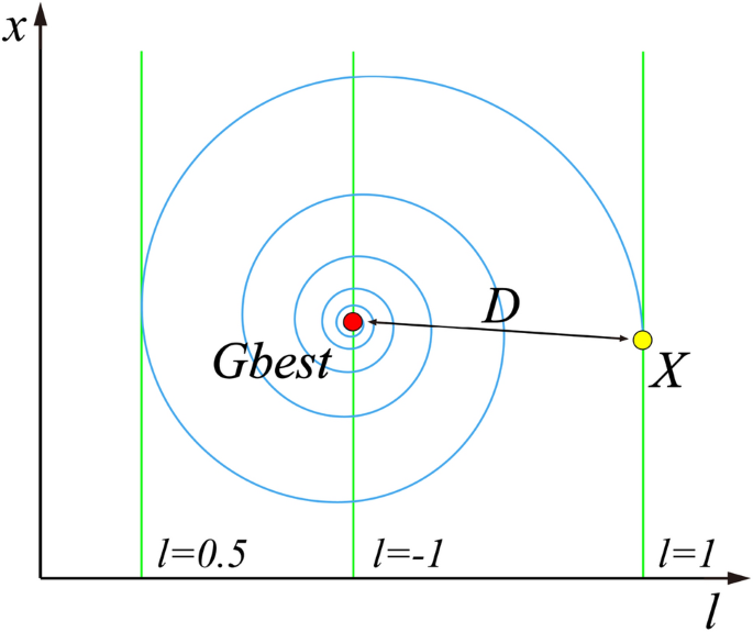
Spiral updating position.

The DE/best/2 mutation strategy is introduced to form the mutant particle. 4 individuals in the population are randomly selected that differ from the current particle, then the vector difference between them is rescaled, and the difference vector is combined with the global optimal position to form the mutant particle. The equation for mutation of particle position is shown as follows:

where \({x}^{*}\) is the mutated particle, \(F\) is the scale factor of mutation, \({r}_{1}\) , \({r}_{2}\) , \({r}_{3}\) , \({r}_{4}\) are random integer values in \((0,n]\) and not equal to \(i\) , respectively. Specific particles are selected for mutation with the screening conditions as follows:

where \(Cr\) represents the probability of mutation, \(rand\left(\mathrm{0,1}\right)\) is a random number in \(\left(\mathrm{0,1}\right)\) , and \({i}_{rand}\) is a random integer value in \((0,n]\) .

The improved PSO incorporates the search ideas of other intelligent algorithms (DE, WOA), so the improved algorithm proposed in this paper is named NDWPSO. The pseudo-code for the NDWPSO algorithm is given as follows:

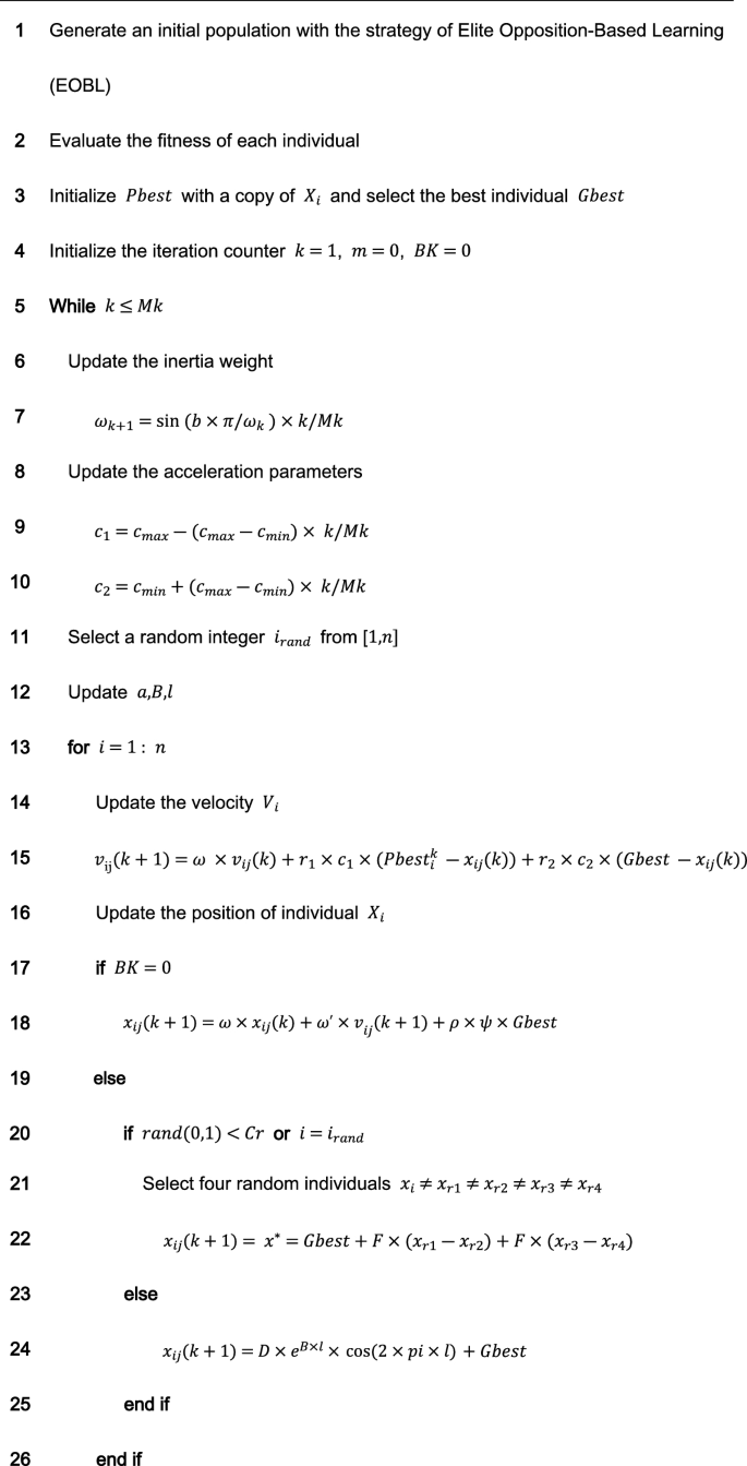
The main procedure of NDWPSO.

Comparing the distribution of inertia weight parameters

There are several improved PSO algorithms (such as CDWPSO 25 , and SDWPSO 26 ) that adopt the dynamic weighted particle position update strategy as their improvement strategy. The updated equations of the CDWPSO and the SDWPSO algorithm for the inertia weight parameters are given as follows:

where \({\text{A}}\) is a value in \((\mathrm{0,1}]\) . \({r}_{max}\) and \({r}_{min}\) are the upper and lower limits of the fluctuation range of the inertia weight parameters, \(k\) is the current number of algorithm iterations, and \(Mk\) denotes the maximum number of iterations.

Considering that the update method of inertia weight parameters by our proposed NDWPSO is comparable to the CDWPSO, and SDWPSO, a comparison experiment for the distribution of inertia weight parameters is set up in this section. The maximum number of iterations in the experiment is \(Mk=500\) . The distributions of CDWPSO, SDWPSO, and NDWPSO inertia weights are shown sequentially in Fig.  2 .

The inertial weight distribution of CDWPSO, SDWPSO, and NDWPSO.

In Fig.  2 , the inertia weight value of CDWPSO is a random value in (0,1]. It may make individual particles fly out of the range in the late iteration of the algorithm. Similarly, the inertia weight value of SDWPSO is a value that tends to zero infinitely, so that the swarm no longer can fly in the search space, making the algorithm extremely easy to fall into the local optimal value. On the other hand, the distribution of the inertia weights of the NDWPSO forms a gentle slope by two curves. Thus, the swarm can faster lock the global optimum range in the early iterations and locate the global optimal more precisely in the late iterations. The reason is that the inertia weight values between two adjacent iterations are inversely proportional to each other. Besides, the time-varying part of the inertial weight within NDWPSO is designed to reduce the chaos characteristic of the parameters. The inertia weight value of NDWPSO avoids the disadvantages of the above two schemes, so its design is more reasonable.

Experiment and discussion

In this section, three experiments are set up to evaluate the performance of NDWPSO: (1) the experiment of 23 classical functions 37 between NDWPSO and three particle swarm algorithms (PSO 6 , CDWPSO 25 , SDWPSO 26 ); (2) the experiment of benchmark test functions between NDWPSO and other intelligent algorithms (Whale Optimization Algorithm (WOA) 36 , Harris Hawk Algorithm (HHO) 38 , Gray Wolf Optimization Algorithm (GWO) 39 , Archimedes Algorithm (AOA) 40 , Equilibrium Optimizer (EO) 41 and Differential Evolution (DE) 42 ); (3) the experiment for solving three real engineering problems (welded beam design 43 , pressure vessel design 44 , and three-bar truss design 38 ). All experiments are run on a computer with Intel i5-11400F GPU, 2.60 GHz, 16 GB RAM, and the code is written with MATLAB R2017b.

The benchmark test functions are 23 classical functions, which consist of indefinite unimodal (F1–F7), indefinite dimensional multimodal functions (F8–F13), and fixed-dimensional multimodal functions (F14–F23). The unimodal benchmark function is used to evaluate the global search performance of different algorithms, while the multimodal benchmark function reflects the ability of the algorithm to escape from the local optimal. The mathematical equations of the benchmark functions are shown and found as Supplementary Tables S1 – S3 online.

Experiments on benchmark functions between NDWPSO, and other PSO variants

The purpose of the experiment is to show the performance advantages of the NDWPSO algorithm. Here, the dimensions and corresponding population sizes of 13 benchmark functions (7 unimodal and 6 multimodal) are set to (30, 40), (50, 70), and (100, 130). The population size of 10 fixed multimodal functions is set to 40. Each algorithm is repeated 30 times independently, and the maximum number of iterations is 200. The performance of the algorithm is measured by the mean and the standard deviation (SD) of the results for different benchmark functions. The parameters of the NDWPSO are set as: \({[{\omega }_{min},\omega }_{max}]=[\mathrm{0.4,0.9}]\) , \(\left[{c}_{max},{c}_{min}\right]=\left[\mathrm{2.5,1.5}\right],{V}_{max}=0.1,b={e}^{-50}, M=0.05\times Mk, B=1,F=0.7, Cr=0.9.\) And, \(A={\omega }_{max}\) for CDWPSO; \({[r}_{max},{r}_{min}]=[\mathrm{4,0}]\) for SDWPSO.

Besides, the experimental data are retained to two decimal places, but some experimental data will increase the number of retained data to pursue more accuracy in comparison. The best results in each group of experiments will be displayed in bold font. The experimental data is set to 0 if the value is below 10 –323 . The experimental parameter settings in this paper are different from the references (PSO 6 , CDWPSO 25 , SDWPSO 26 , so the final experimental data differ from the ones within the reference.

As shown in Tables 1 and 2 , the NDWPSO algorithm obtains better results for all 49 sets of data than other PSO variants, which include not only 13 indefinite-dimensional benchmark functions and 10 fixed-multimodal benchmark functions. Remarkably, the SDWPSO algorithm obtains the same accuracy of calculation as NDWPSO for both unimodal functions f 1 –f 4 and multimodal functions f 9 –f 11 . The solution accuracy of NDWPSO is higher than that of other PSO variants for fixed-multimodal benchmark functions f 14 -f 23 . The conclusion can be drawn that the NDWPSO has excellent global search capability, local search capability, and the capability for escaping the local optimal.

In addition, the convergence curves of the 23 benchmark functions are shown in Figs. 3 , 4 , 5 , 6 , 7 , 8 , 9 , 10 , 11 , 12 , 13 , 14 , 15 , 16 , 17 , 18 and 19 . The NDWPSO algorithm has a faster convergence speed in the early stage of the search for processing functions f1-f6, f8-f14, f16, f17, and finds the global optimal solution with a smaller number of iterations. In the remaining benchmark function experiments, the NDWPSO algorithm shows no outstanding performance for convergence speed in the early iterations. There are two reasons of no outstanding performance in the early iterations. On one hand, the fixed-multimodal benchmark function has many disturbances and local optimal solutions in the whole search space. on the other hand, the initialization scheme based on elite opposition-based learning is still stochastic, which leads to the initial position far from the global optimal solution. The inertia weight based on chaotic mapping and the strategy of spiral updating can significantly improve the convergence speed and computational accuracy of the algorithm in the late search stage. Finally, the NDWPSO algorithm can find better solutions than other algorithms in the middle and late stages of the search.

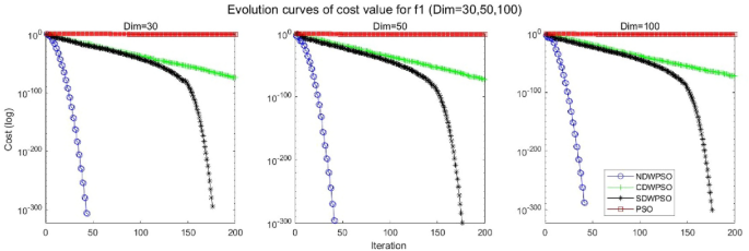
Evolution curve of NDWPSO and other PSO algorithms for f1 (Dim = 30,50,100).

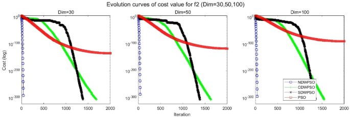
Evolution curve of NDWPSO and other PSO algorithms for f2 (Dim = 30,50,100).

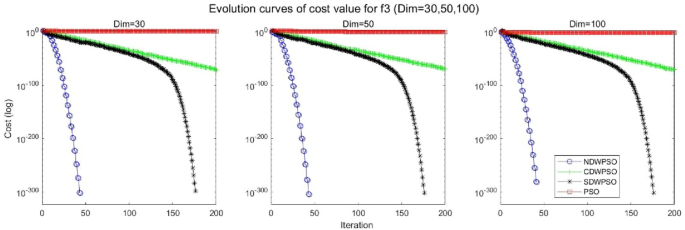
Evolution curve of NDWPSO and other PSO algorithms for f3 (Dim = 30,50,100).

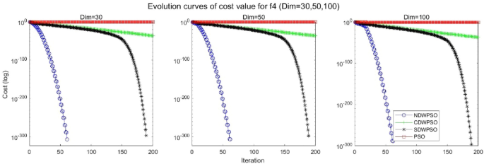
Evolution curve of NDWPSO and other PSO algorithms for f4 (Dim = 30,50,100).

Evolution curve of NDWPSO and other PSO algorithms for f5 (Dim = 30,50,100).

Evolution curve of NDWPSO and other PSO algorithms for f6 (Dim = 30,50,100).

Evolution curve of NDWPSO and other PSO algorithms for f7 (Dim = 30,50,100).

Evolution curve of NDWPSO and other PSO algorithms for f8 (Dim = 30,50,100).

Evolution curve of NDWPSO and other PSO algorithms for f9 (Dim = 30,50,100).

Evolution curve of NDWPSO and other PSO algorithms for f10 (Dim = 30,50,100).

Evolution curve of NDWPSO and other PSO algorithms for f11(Dim = 30,50,100).

Evolution curve of NDWPSO and other PSO algorithms for f12 (Dim = 30,50,100).

Evolution curve of NDWPSO and other PSO algorithms for f13 (Dim = 30,50,100).

Evolution curve of NDWPSO and other PSO algorithms for f14, f15, f16.

Evolution curve of NDWPSO and other PSO algorithms for f17, f18, f19.

Evolution curve of NDWPSO and other PSO algorithms for f20, f21, f22.

Evolution curve of NDWPSO and other PSO algorithms for f23.

To evaluate the performance of different PSO algorithms, a statistical test is conducted. Due to the stochastic nature of the meta-heuristics, it is not enough to compare algorithms based on only the mean and standard deviation values. The optimization results cannot be assumed to obey the normal distribution; thus, it is necessary to judge whether the results of the algorithms differ from each other in a statistically significant way. Here, the Wilcoxon non-parametric statistical test 45 is used to obtain a parameter called p -value to verify whether two sets of solutions are different to a statistically significant extent or not. Generally, it is considered that p  ≤ 0.5 can be considered as a statistically significant superiority of the results. The p -values calculated in Wilcoxon’s rank-sum test comparing NDWPSO and other PSO algorithms are listed in Table  3 for all benchmark functions. The p -values in Table  3 additionally present the superiority of the NDWPSO because all of the p -values are much smaller than 0.5.

In general, the NDWPSO has the fastest convergence rate when finding the global optimum from Figs. 3 , 4 , 5 , 6 , 7 , 8 , 9 , 10 , 11 , 12 , 13 , 14 , 15 , 16 , 17 , 18 and 19 , and thus we can conclude that the NDWPSO is superior to the other PSO variants during the process of optimization.

Comparison experiments between NDWPSO and other intelligent algorithms

Experiments are conducted to compare NDWPSO with several other intelligent algorithms (WOA, HHO, GWO, AOA, EO and DE). The experimental object is 23 benchmark functions, and the experimental parameters of the NDWPSO algorithm are set the same as in Experiment 4.1. The maximum number of iterations of the experiment is increased to 2000 to fully demonstrate the performance of each algorithm. Each algorithm is repeated 30 times individually. The parameters of the relevant intelligent algorithms in the experiments are set as shown in Table 4 . To ensure the fairness of the algorithm comparison, all parameters are concerning the original parameters in the relevant algorithm literature. The experimental results are shown in Tables 5 , 6 , 7 and 8 and Figs. 20 , 21 , 22 , 23 , 24 , 25 , 26 , 27 , 28 , 29 , 30 , 31 , 32 , 33 , 34 , 35 and 36 .

Evolution curve of NDWPSO and other algorithms for f1 (Dim = 30,50,100).

Evolution curve of NDWPSO and other algorithms for f2 (Dim = 30,50,100).

Evolution curve of NDWPSO and other algorithms for f3(Dim = 30,50,100).

Evolution curve of NDWPSO and other algorithms for f4 (Dim = 30,50,100).

Evolution curve of NDWPSO and other algorithms for f5 (Dim = 30,50,100).

Evolution curve of NDWPSO and other algorithms for f6 (Dim = 30,50,100).

Evolution curve of NDWPSO and other algorithms for f7 (Dim = 30,50,100).

Evolution curve of NDWPSO and other algorithms for f8 (Dim = 30,50,100).

Evolution curve of NDWPSO and other algorithms for f9(Dim = 30,50,100).

Evolution curve of NDWPSO and other algorithms for f10 (Dim = 30,50,100).

Evolution curve of NDWPSO and other algorithms for f11 (Dim = 30,50,100).

Evolution curve of NDWPSO and other algorithms for f12 (Dim = 30,50,100).

Evolution curve of NDWPSO and other algorithms for f13 (Dim = 30,50,100).

Evolution curve of NDWPSO and other algorithms for f14, f15, f16.

Evolution curve of NDWPSO and other algorithms for f17, f18, f19.

Evolution curve of NDWPSO and other algorithms for f20, f21, f22.

Evolution curve of NDWPSO and other algorithms for f23.

The experimental data of NDWPSO and other intelligent algorithms for handling 30, 50, and 100-dimensional benchmark functions ( \({f}_{1}-{f}_{13}\) ) are recorded in Tables 8 , 9 and 10 , respectively. The comparison data of fixed-multimodal benchmark tests ( \({f}_{14}-{f}_{23}\) ) are recorded in Table 11 . According to the data in Tables 5 , 6 and 7 , the NDWPSO algorithm obtains 69.2%, 84.6%, and 84.6% of the best results for the benchmark function ( \({f}_{1}-{f}_{13}\) ) in the search space of three dimensions (Dim = 30, 50, 100), respectively. In Table 8 , the NDWPSO algorithm obtains 80% of the optimal solutions in 10 fixed-multimodal benchmark functions.

The convergence curves of each algorithm are shown in Figs. 20 , 21 , 22 , 23 , 24 , 25 , 26 , 27 , 28 , 29 , 30 , 31 , 32 , 33 , 34 , 35 and 36 . The NDWPSO algorithm demonstrates two convergence behaviors when calculating the benchmark functions in 30, 50, and 100-dimensional search spaces. The first behavior is the fast convergence of NDWPSO with a small number of iterations at the beginning of the search. The reason is that the Iterative-mapping strategy and the position update scheme of dynamic weighting are used in the NDWPSO algorithm. This scheme can quickly target the region in the search space where the global optimum is located, and then precisely lock the optimal solution. When NDWPSO processes the functions \({f}_{1}-{f}_{4}\) , and \({f}_{9}-{f}_{11}\) , the behavior can be reflected in the convergence trend of their corresponding curves. The second behavior is that NDWPSO gradually improves the convergence accuracy and rapidly approaches the global optimal in the middle and late stages of the iteration. The NDWPSO algorithm fails to converge quickly in the early iterations, which is possible to prevent the swarm from falling into a local optimal. The behavior can be demonstrated by the convergence trend of the curves when NDWPSO handles the functions \({f}_{6}\) , \({f}_{12}\) , and \({f}_{13}\) , and it also shows that the NDWPSO algorithm has an excellent ability of local search.

Combining the experimental data with the convergence curves, it is concluded that the NDWPSO algorithm has a faster convergence speed, so the effectiveness and global convergence of the NDWPSO algorithm are more outstanding than other intelligent algorithms.

Experiments on classical engineering problems

Three constrained classical engineering design problems (welded beam design, pressure vessel design 43 , and three-bar truss design 38 ) are used to evaluate the NDWPSO algorithm. The experiments are the NDWPSO algorithm and 5 other intelligent algorithms (WOA 36 , HHO, GWO, AOA, EO 41 ). Each algorithm is provided with the maximum number of iterations and population size ( \({\text{Mk}}=500,\mathrm{ n}=40\) ), and then repeats 30 times, independently. The parameters of the algorithms are set the same as in Table 4 . The experimental results of three engineering design problems are recorded in Tables 9 , 10 and 11 in turn. The result data is the average value of the solved data.

Welded beam design

The target of the welded beam design problem is to find the optimal manufacturing cost for the welded beam with the constraints, as shown in Fig.  37 . The constraints are the thickness of the weld seam ( \({\text{h}}\) ), the length of the clamped bar ( \({\text{l}}\) ), the height of the bar ( \({\text{t}}\) ) and the thickness of the bar ( \({\text{b}}\) ). The mathematical formulation of the optimization problem is given as follows:

Welded beam design.

In Table 9 , the NDWPSO, GWO, and EO algorithms obtain the best optimal cost. Besides, the standard deviation (SD) of t NDWPSO is the lowest, which means it has very good results in solving the welded beam design problem.

Pressure vessel design

Kannan and Kramer 43 proposed the pressure vessel design problem as shown in Fig.  38 to minimize the total cost, including the cost of material, forming, and welding. There are four design optimized objects: the thickness of the shell \({T}_{s}\) ; the thickness of the head \({T}_{h}\) ; the inner radius \({\text{R}}\) ; the length of the cylindrical section without considering the head \({\text{L}}\) . The problem includes the objective function and constraints as follows:

Pressure vessel design.

The results in Table 10 show that the NDWPSO algorithm obtains the lowest optimal cost with the same constraints and has the lowest standard deviation compared with other algorithms, which again proves the good performance of NDWPSO in terms of solution accuracy.

Three-bar truss design

This structural design problem 44 is one of the most widely-used case studies as shown in Fig.  39 . There are two main design parameters: the area of the bar1 and 3 ( \({A}_{1}={A}_{3}\) ) and area of bar 2 ( \({A}_{2}\) ). The objective is to minimize the weight of the truss. This problem is subject to several constraints as well: stress, deflection, and buckling constraints. The problem is formulated as follows:

Three-bar truss design.

From Table 11 , NDWPSO obtains the best design solution in this engineering problem and has the smallest standard deviation of the result data. In summary, the NDWPSO can reveal very competitive results compared to other intelligent algorithms.

Conclusions and future works

An improved algorithm named NDWPSO is proposed to enhance the solving speed and improve the computational accuracy at the same time. The improved NDWPSO algorithm incorporates the search ideas of other intelligent algorithms (DE, WOA). Besides, we also proposed some new hybrid strategies to adjust the distribution of algorithm parameters (such as the inertia weight parameter, the acceleration coefficients, the initialization scheme, the position updating equation, and so on).

23 classical benchmark functions: indefinite unimodal (f1-f7), indefinite multimodal (f8-f13), and fixed-dimensional multimodal(f14-f23) are applied to evaluate the effective line and feasibility of the NDWPSO algorithm. Firstly, NDWPSO is compared with PSO, CDWPSO, and SDWPSO. The simulation results can prove the exploitative, exploratory, and local optima avoidance of NDWPSO. Secondly, the NDWPSO algorithm is compared with 5 other intelligent algorithms (WOA, HHO, GWO, AOA, EO). The NDWPSO algorithm also has better performance than other intelligent algorithms. Finally, 3 classical engineering problems are applied to prove that the NDWPSO algorithm shows superior results compared to other algorithms for the constrained engineering optimization problems.

Although the proposed NDWPSO is superior in many computation aspects, there are still some limitations and further improvements are needed. The NDWPSO performs a limit initialize on each particle by the strategy of “elite opposition-based learning”, it takes more computation time before speed update. Besides, the” local optimal jump-out” strategy also brings some random process. How to reduce the random process and how to improve the limit initialize efficiency are the issues that need to be further discussed. In addition, in future work, researchers will try to apply the NDWPSO algorithm to wider fields to solve more complex and diverse optimization problems.

Data availability

The datasets used and/or analyzed during the current study available from the corresponding author on reasonable request.

Sami, F. Optimize electric automation control using artificial intelligence (AI). Optik 271 , 170085 (2022).

Article   ADS   Google Scholar  

Li, X. et al. Prediction of electricity consumption during epidemic period based on improved particle swarm optimization algorithm. Energy Rep. 8 , 437–446 (2022).

Article   Google Scholar  

Sun, B. Adaptive modified ant colony optimization algorithm for global temperature perception of the underground tunnel fire. Case Stud. Therm. Eng. 40 , 102500 (2022).

Bartsch, G. et al. Use of artificial intelligence and machine learning algorithms with gene expression profiling to predict recurrent nonmuscle invasive urothelial carcinoma of the bladder. J. Urol. 195 (2), 493–498 (2016).

Article   PubMed   Google Scholar  

Bao, Z. Secure clustering strategy based on improved particle swarm optimization algorithm in internet of things. Comput. Intell. Neurosci. 2022 , 1–9 (2022).

Google Scholar  

Kennedy, J. & Eberhart, R. Particle swarm optimization. In: Proceedings of ICNN'95-International Conference on Neural Networks . IEEE, 1942–1948 (1995).

Lin, Q. et al. A novel artificial bee colony algorithm with local and global information interaction. Appl. Soft Comput. 62 , 702–735 (2018).

Abed-alguni, B. H. et al. Exploratory cuckoo search for solving single-objective optimization problems. Soft Comput. 25 (15), 10167–10180 (2021).

Brajević, I. A shuffle-based artificial bee colony algorithm for solving integer programming and minimax problems. Mathematics 9 (11), 1211 (2021).

Khan, A. T. et al. Non-linear activated beetle antennae search: A novel technique for non-convex tax-aware portfolio optimization problem. Expert Syst. Appl. 197 , 116631 (2022).

Brajević, I. et al. Hybrid sine cosine algorithm for solving engineering optimization problems. Mathematics 10 (23), 4555 (2022).

Abed-Alguni, B. H., Paul, D. & Hammad, R. Improved Salp swarm algorithm for solving single-objective continuous optimization problems. Appl. Intell. 52 (15), 17217–17236 (2022).

Nadimi-Shahraki, M. H. et al. Binary starling murmuration optimizer algorithm to select effective features from medical data. Appl. Sci. 13 (1), 564 (2022).

Nadimi-Shahraki, M. H. et al. A systematic review of the whale optimization algorithm: Theoretical foundation, improvements, and hybridizations. Archiv. Comput. Methods Eng. 30 (7), 4113–4159 (2023).

Fatahi, A., Nadimi-Shahraki, M. H. & Zamani, H. An improved binary quantum-based avian navigation optimizer algorithm to select effective feature subset from medical data: A COVID-19 case study. J. Bionic Eng. 21 (1), 426–446 (2024).

Abed-alguni, B. H. & AL-Jarah, S. H. IBJA: An improved binary DJaya algorithm for feature selection. J. Comput. Sci. 75 , 102201 (2024).

Yeh, W.-C. A novel boundary swarm optimization method for reliability redundancy allocation problems. Reliab. Eng. Syst. Saf. 192 , 106060 (2019).

Solomon, S., Thulasiraman, P. & Thulasiram, R. Collaborative multi-swarm PSO for task matching using graphics processing units. In: Proceedings of the 13th Annual Conference on Genetic and Evolutionary Computation 1563–1570 (2011).

Mukhopadhyay, S. & Banerjee, S. Global optimization of an optical chaotic system by chaotic multi swarm particle swarm optimization. Expert Syst. Appl. 39 (1), 917–924 (2012).

Duan, L. et al. Improved particle swarm optimization algorithm for enhanced coupling of coaxial optical communication laser. Opt. Fiber Technol. 64 , 102559 (2021).

Sun, F., Xu, Z. & Zhang, D. Optimization design of wind turbine blade based on an improved particle swarm optimization algorithm combined with non-gaussian distribution. Adv. Civ. Eng. 2021 , 1–9 (2021).

Liu, M. et al. An improved particle-swarm-optimization algorithm for a prediction model of steel slab temperature. Appl. Sci. 12 (22), 11550 (2022).

Article   MathSciNet   CAS   Google Scholar  

Gad, A. G. Particle swarm optimization algorithm and its applications: A systematic review. Archiv. Comput. Methods Eng. 29 (5), 2531–2561 (2022).

Article   MathSciNet   Google Scholar  

Feng, H. et al. Trajectory control of electro-hydraulic position servo system using improved PSO-PID controller. Autom. Constr. 127 , 103722 (2021).

Chen, Ke., Zhou, F. & Liu, A. Chaotic dynamic weight particle swarm optimization for numerical function optimization. Knowl. Based Syst. 139 , 23–40 (2018).

Bai, B. et al. Reliability prediction-based improved dynamic weight particle swarm optimization and back propagation neural network in engineering systems. Expert Syst. Appl. 177 , 114952 (2021).

Alsaidy, S. A., Abbood, A. D. & Sahib, M. A. Heuristic initialization of PSO task scheduling algorithm in cloud computing. J. King Saud Univ. –Comput. Inf. Sci. 34 (6), 2370–2382 (2022).

Liu, H., Cai, Z. & Wang, Y. Hybridizing particle swarm optimization with differential evolution for constrained numerical and engineering optimization. Appl. Soft Comput. 10 (2), 629–640 (2010).

Deng, W. et al. A novel intelligent diagnosis method using optimal LS-SVM with improved PSO algorithm. Soft Comput. 23 , 2445–2462 (2019).

Huang, M. & Zhen, L. Research on mechanical fault prediction method based on multifeature fusion of vibration sensing data. Sensors 20 (1), 6 (2019).

Article   ADS   PubMed   PubMed Central   Google Scholar  

Wolpert, D. H. & Macready, W. G. No free lunch theorems for optimization. IEEE Trans. Evol. Comput. 1 (1), 67–82 (1997).

Gandomi, A. H. et al. Firefly algorithm with chaos. Commun. Nonlinear Sci. Numer. Simul. 18 (1), 89–98 (2013).

Article   ADS   MathSciNet   Google Scholar  

Zhou, Y., Wang, R. & Luo, Q. Elite opposition-based flower pollination algorithm. Neurocomputing 188 , 294–310 (2016).

Li, G., Niu, P. & Xiao, X. Development and investigation of efficient artificial bee colony algorithm for numerical function optimization. Appl. Soft Comput. 12 (1), 320–332 (2012).

Xiong, G. et al. Parameter extraction of solar photovoltaic models by means of a hybrid differential evolution with whale optimization algorithm. Solar Energy 176 , 742–761 (2018).

Mirjalili, S. & Lewis, A. The whale optimization algorithm. Adv. Eng. Softw. 95 , 51–67 (2016).

Yao, X., Liu, Y. & Lin, G. Evolutionary programming made faster. IEEE Trans. Evol. Comput. 3 (2), 82–102 (1999).

Heidari, A. A. et al. Harris hawks optimization: Algorithm and applications. Fut. Gener. Comput. Syst. 97 , 849–872 (2019).

Mirjalili, S., Mirjalili, S. M. & Lewis, A. Grey wolf optimizer. Adv. Eng. Softw. 69 , 46–61 (2014).

Hashim, F. A. et al. Archimedes optimization algorithm: A new metaheuristic algorithm for solving optimization problems. Appl. Intell. 51 , 1531–1551 (2021).

Faramarzi, A. et al. Equilibrium optimizer: A novel optimization algorithm. Knowl. -Based Syst. 191 , 105190 (2020).

Pant, M. et al. Differential evolution: A review of more than two decades of research. Eng. Appl. Artif. Intell. 90 , 103479 (2020).

Coello, C. A. C. Use of a self-adaptive penalty approach for engineering optimization problems. Comput. Ind. 41 (2), 113–127 (2000).

Kannan, B. K. & Kramer, S. N. An augmented lagrange multiplier based method for mixed integer discrete continuous optimization and its applications to mechanical design. J. Mech. Des. 116 , 405–411 (1994).

Derrac, J. et al. A practical tutorial on the use of nonparametric statistical tests as a methodology for comparing evolutionary and swarm intelligence algorithms. Swarm Evol. Comput. 1 (1), 3–18 (2011).

Download references

Acknowledgements

This work was supported by Key R&D plan of Shandong Province, China (2021CXGC010207, 2023CXGC01020); First batch of talent research projects of Qilu University of Technology in 2023 (2023RCKY116); Introduction of urgently needed talent projects in Key Supported Regions of Shandong Province; Key Projects of Natural Science Foundation of Shandong Province (ZR2020ME116); the Innovation Ability Improvement Project for Technology-based Small- and Medium-sized Enterprises of Shandong Province (2022TSGC2051, 2023TSGC0024, 2023TSGC0931); National Key R&D Program of China (2019YFB1705002), LiaoNing Revitalization Talents Program (XLYC2002041) and Young Innovative Talents Introduction & Cultivation Program for Colleges and Universities of Shandong Province (Granted by Department of Education of Shandong Province, Sub-Title: Innovative Research Team of High Performance Integrated Device).

Author information

Authors and affiliations.

School of Mechanical and Automotive Engineering, Qilu University of Technology (Shandong Academy of Sciences), Jinan, 250353, China

Jinwei Qiao, Guangyuan Wang, Zhi Yang, Jun Chen & Pengbo Liu

Shandong Institute of Mechanical Design and Research, Jinan, 250353, China

School of Information Science and Engineering, Northeastern University, Shenyang, 110819, China

Xiaochuan Luo

Fushun Supervision Inspection Institute for Special Equipment, Fushun, 113000, China

You can also search for this author in PubMed   Google Scholar

Contributions

Z.Y., J.Q., and G.W. wrote the main manuscript text and prepared all figures and tables. J.C., P.L., K.L., and X.L. were responsible for the data curation and software. All authors reviewed the manuscript.

Corresponding author

Correspondence to Zhi Yang .

Ethics declarations

Competing interests.

The authors declare no competing interests.

Additional information

Publisher's note.

Springer Nature remains neutral with regard to jurisdictional claims in published maps and institutional affiliations.

Supplementary Information

Supplementary information., rights and permissions.

Open Access This article is licensed under a Creative Commons Attribution 4.0 International License, which permits use, sharing, adaptation, distribution and reproduction in any medium or format, as long as you give appropriate credit to the original author(s) and the source, provide a link to the Creative Commons licence, and indicate if changes were made. The images or other third party material in this article are included in the article's Creative Commons licence, unless indicated otherwise in a credit line to the material. If material is not included in the article's Creative Commons licence and your intended use is not permitted by statutory regulation or exceeds the permitted use, you will need to obtain permission directly from the copyright holder. To view a copy of this licence, visit http://creativecommons.org/licenses/by/4.0/ .

Reprints and permissions

About this article

Cite this article.

Qiao, J., Wang, G., Yang, Z. et al. A hybrid particle swarm optimization algorithm for solving engineering problem. Sci Rep 14 , 8357 (2024). https://doi.org/10.1038/s41598-024-59034-2

Download citation

Received : 11 January 2024

Accepted : 05 April 2024

Published : 10 April 2024

DOI : https://doi.org/10.1038/s41598-024-59034-2

Share this article

Anyone you share the following link with will be able to read this content:

Sorry, a shareable link is not currently available for this article.

Provided by the Springer Nature SharedIt content-sharing initiative

• Particle swarm optimization
• Elite opposition-based learning
• Iterative mapping
• Convergence analysis

By submitting a comment you agree to abide by our Terms and Community Guidelines . If you find something abusive or that does not comply with our terms or guidelines please flag it as inappropriate.

Quick links

• Explore articles by subject
• Guide to authors
• Editorial policies

Sign up for the Nature Briefing: AI and Robotics newsletter — what matters in AI and robotics research, free to your inbox weekly.

Secretary bird optimization algorithm: a new metaheuristic for solving global optimization problems

• Open access
• Published: 23 April 2024
• Volume 57 , article number  123 , ( 2024 )

Cite this article

You have full access to this open access article

• Youfa Fu 1 ,
• Dan Liu 1 ,
• Jiadui Chen 1 &
• Ling He 1  

This study introduces a novel population-based metaheuristic algorithm called secretary bird optimization algorithm (SBOA), inspired by the survival behavior of secretary birds in their natural environment. Survival for secretary birds involves continuous hunting for prey and evading pursuit from predators. This information is crucial for proposing a new metaheuristic algorithm that utilizes the survival abilities of secretary birds to address real-world optimization problems. The algorithm's exploration phase simulates secretary birds hunting snakes, while the exploitation phase models their escape from predators. During this phase, secretary birds observe the environment and choose the most suitable way to reach a secure refuge. These two phases are iteratively repeated, subject to termination criteria, to find the optimal solution to the optimization problem. To validate the performance of SBOA, experiments were conducted to assess convergence speed, convergence behavior, and other relevant aspects. Furthermore, we compared SBOA with 15 advanced algorithms using the CEC-2017 and CEC-2022 benchmark suites. All test results consistently demonstrated the outstanding performance of SBOA in terms of solution quality, convergence speed, and stability. Lastly, SBOA was employed to tackle 12 constrained engineering design problems and perform three-dimensional path planning for Unmanned Aerial Vehicles. The results demonstrate that, compared to contrasted optimizers, the proposed SBOA can find better solutions at a faster pace, showcasing its significant potential in addressing real-world optimization problems.

Avoid common mistakes on your manuscript.

1 Introduction

With the continuous development of society and technology, optimization problems have become increasingly complex and challenging in various domains. The nature of these problems encompasses a wide range of areas, including manufacturing, resource allocation, path planning, financial portfolio optimization, and others. They involve multiple decision variables, numerous constraints, and diverse objective functions. In the face of real-world constraints such as resource scarcity, cost control, and efficiency requirements, finding optimal solutions has become an urgent imperative (Zhou et al. 2011 ).

Traditional mathematical optimization methods, while performing well in certain cases, often exhibit limitations when dealing with complex, high-dimensional, nonlinear, and multimodal problems. Issues such as local optima, slow convergence rates, difficulty in parameter tuning, high-dimensional problems, and computational costs have been persistent challenges for researchers and practitioners in the field of optimization (Faramarzi et al. 2020b ). Therefore, people are seeking new methods and technologies to address these challenges. In this context, metaheuristic algorithms have emerged. They belong to a category of intelligent search algorithms inspired by natural phenomena and mechanisms, designed to find solutions to optimization problems through stochastic methods. Unlike traditional mathematical optimization methods, metaheuristic algorithms are better suited for complex, multimodal, high-dimensional, and nonlinear optimization problems. These algorithms, by simulating processes like evolution, swarm intelligence, and simulated annealing found in nature, exhibit robustness and global search capabilities, and as a result, they have gained widespread popularity in various practical applications.

Despite the significant progress that metaheuristic algorithms have made in various fields, they also face some challenges and issues, including susceptibility to getting stuck in local optima, slow convergence rates, insufficient robustness, and high computational costs (Agrawal et al. 2021 ). Despite the significant progress that metaheuristic algorithms have made in various fields, they also face some challenges and issues, including susceptibility to getting stuck in local optima, slow convergence rates, insufficient robustness, and high computational costs (Wolpert and Macready 1997 ) explicitly stated that the significant performance of an algorithm in solving a specific set of optimization problems does not guarantee that it will perform equally well in other optimization problems. Therefore, not all algorithms excel at in all optimization applications. The NFL theorem drives researchers to design innovative algorithms that can more effectively solve optimization problems by providing better solutions. In certain scenarios, algorithmic convergence to local optima may occur due to an imbalance between development and exploration. To address this issue, various approaches have been proposed. Nama et al. introduced a novel integrated algorithm, denoted as e-mPSOBSA (Nama et al. 2023 ), based on the Backtracking Search Algorithm (BSA) and Particle Swarm Optimization (PSO). This integration aims to mitigate the imbalance between development and exploration. Nama et al. proposed an improved version of the Backtracking Search Algorithm, named gQR-BSA (Nama et al. 2022b ), to address challenges arising from the imbalance between exploitation and exploration. He presented a bio-inspired multi-population self-adaptive Backtracking Search Algorithm, referred to as ImBSA (Nama and Saha 2022 ), as a solution to the development-exploration imbalance. Nama presented an enhanced symbiotic organism search algorithm, mISOS (Nama 2021 ), to overcome challenges associated with development-exploration imbalance. Chakraborty introduced an enhanced version of the Symbiotic Organism Search algorithm, namely nwSOS (Chakraborty et al. 2022a ), designed for solving optimization problems in higher dimensions. Saha combined the exploration capability of SQI with the development potential of SOS, proposing the hybrid symbiotic organism search (HSOS) algorithm (Saha et al. 2021 ) and a new parameter setting-based modified differential evolution for function optimization (Nama and Saha 2020 ). This combination enhances the algorithm's robustness and overall performance.

Engineering optimization problems have consistently posed significant challenges within the field of engineering. These problems involve achieving specific objectives, typically involve cost minimization, efficiency maximization, or performance optimization, under limited resources. The challenges in engineering optimization arise from their diversity and complexity. Problems can be either discrete or continuous, involve multiple decision variables, are subject to various constraints, and may incorporate elements of randomness and uncertainty. Consequently, selecting appropriate optimization algorithms is crucial for solving these problems. In recent decades, researchers have developed various types of optimization algorithms, including traditional mathematical programming methods, heuristic algorithms, and evolutionary algorithms, among others. However, these algorithms still exhibit certain limitations when addressing such optimization problems. For example, when dealing with more complex problems, they tend to have slow convergence rates, limited search precision, and are prone to becoming trapped in local optima.

To overcome these challenges, this paper introduces a new optimization algorithm—the secretary bird optimization algorithm (SBOA). Our motivation is to address the shortcomings of existing algorithms in tackling complex engineering optimization problems. Specifically, our focus lies in improving the convergence speed of optimization algorithms, enhancing optimization precision, and effectively avoiding local optima. By introducing the secretary bird optimization algorithm, we aim to provide a more efficient and reliable solution for the engineering domain, fostering new breakthroughs in the research and practical application of optimization problems. The primary contributions of this study are as follows:

Introduced a novel population-based metaheuristic algorithm named secretary bird optimization algorithm (SBOA), which is designed to simulate the survival capabilities of secretary birds in their natural environment.

SBOA is inspired by the hunting and evading abilities of secretary birds in dealing with predators, where survival adaptability is divided into two phases: exploration and exploitation.

The exploration phase of the algorithm simulates the behavior of secretary birds capturing snakes, while the exploitation phase simulates their behavior of evading predators.

Mathematical modeling is employed to describe and analyze each stage of SBOA.

Evaluate the effectiveness and robustness of SBOA by solving 42 benchmark functions, including unimodal, multimodal, hybrid, and composition functions defined in CEC 2017, and CEC 2022.

The performance of SBOA in solving practical optimization problems is tested on twelve engineering optimization design problems and three-dimensional path planning for unmanned aerial vehicles (UAVs).

The structure of this paper is arranged as follows: the literature review is presented in Sect.  2 . Section  3 introduces the proposed SBOA and models it. Section  4 presents a simulation analysis of the convergence behavior, the exploration and exploitation balance ratio and search agent distribution of SBOA when dealing with optimization problems. Section  5 uses twelve engineering optimization problems to verify the efficiency of SBOA in solving practical engineering optimization problems and addresses a path planning scenario for an unmanned aerial vehicles (UAVs). Section  6 provides the conclusion and outlines several directions for future research.

2 Literature review

Metaheuristic algorithms, as a branch of bio-inspired methods, have been widely employed to solve problems in various domains. These algorithms can be classified into several categories based on their underlying principles, including evolutionary algorithms (EA), physics-inspired algorithms (PhA), human behavior-based algorithms, and swarm intelligence (SI) algorithms (Abualigah et al. 2021 ). EA draws inspiration from natural evolutionary processes, with genetic algorithms (GA) (Holland 1992 ) and differential evolution (DE) (Storn and Price 1997 ) as two of its most representative members. These algorithms are rooted in Darwin's theory of evolution. On the other hand, PhA are often inspired by physical phenomena. A notable example is the simulated annealing algorithm (SA) (Kirkpatrick et al. 1983 ), which simulates the annealing process of solids. It uses this physical analogy to find optimal solutions. Human behavior-based algorithms are based on the principles of human social learning. A typical example is the social evolution and learning optimization algorithm (SELOA) (Kumar et al. 2018 ). SI algorithms are inspired by the collective behavior of biological populations in nature. Particle swarm optimization (PSO) (Kennedy and Eberhart 1995 ) is one such algorithm that mimics the foraging behavior of birds. In PSO, particles represent birds searching for food (the objective function) in the forest (search space). During each iteration, particle movement is influenced by both individual and group-level information. Ultimately, particles converge toward the best solution in their vicinity.

The laws of physics play a crucial role in the PhA algorithm, providing essential guidance for optimizing problem solutions. For instance, the simulated annealing algorithm (SA) (Kirkpatrick et al. 1983 ) draws inspiration from the physical phenomenon of metal melting and its cooling and solidification process. The homonuclear molecular orbital (HMO) optimization (HMO) (Mahdavi-Meymand and Zounemat-Kermani 2022 ) is proposed based on the Bohr atomic model and the electron arrangement behavior around the atomic nucleus in the context of the homonuclear molecular structure. Additionally, the special relativity search (SRS) (Goodarzimehr et al. 2022 ) is introduced by applying concepts from electromagnetism and the theory of special relativity. The gravity search algorithm (GSA) (Rashedi et al. 2009 ) is based on Newton's universal law of gravitation. The subtraction-average-based optimizer (SABO) (Trojovský and Dehghani 2023 ) is inspired by mathematical concepts such as the mean, differences in search agent positions, and differences in the values of the objective function. The big bang-big crunch algorithm (BB-BC) (Erol and Eksin 2006 ) is based on Newton's universal law of gravitation. The big bang-big crunch algorithm (BB-BC) (Mirjalili et al. 2016 ), water cycle algorithm (WCA)(Eskandar et al. 2012 ), nuclear reaction optimization (NRO) (Wei et al. 2019 ), nuclear reaction optimization (NRO) (Kaveh and Khayatazad 2012 ). Sinh Cosh optimizer (SCHO) (Bai et al. 2023 ) is inspired by the mathematical characteristics of the hyperbolic sine (Sinh) and hyperbolic cosine (Cosh) functions. The great wall construction algorithm (GWCA) (Guan et al. 2023 ) is inspired by the competitive and elimination mechanisms among workers during the construction of the Great Wall. The exponential distribution optimizer (EDO) (Abdel-Basset et al. 2023a ) is based on the mathematical model of exponential probability distribution. Snowmelt optimizer (SAO) (Deng and Liu 2023 ) inspired by the sublimation and melting behavior of snow in the natural world. The optical microscope algorithm (OMA) (Cheng and Sholeh 2023 ) is inspired by the magnification capability of optical microscopes when observing target objects. It involves a preliminary observation with the naked eye and is further inspired by the simulated magnification process using objective and eyepiece lenses, and rime optimizer (RIME) (Su et al. 2023 ) inspired by the mechanism of ice growth in haze, also draw insights from various physical phenomena.

The MH algorithm, which is based on human behavior, aims to solve optimization problems by simulating some natural behaviors of humans. For instance, the teaching and learning-based optimization algorithm (TBLA) (Rao et al. 2011 ) The MH algorithm, which is based on human behavior, aims to solve optimization problems by simulating some natural behaviors of humans. For instance, the teaching and learning-based optimization algorithm (TBLA) (Kumar et al. 2018 ), which is developed by simulating the social learning behaviors of humans in societal settings, particularly in family organizations. A proposed an improved approach to Teaching–Learning-Based Optimization, referred to as Hybrid Teaching–Learning-Based Optimization (Nama et al. 2020 ).The human evolutionary optimization algorithm (HEOA) (Lian and Hui 2024 ) draws inspiration from human evolution. HEOA divides the global search process into two distinct stages: human exploration and human development. Logical chaotic mapping is used for initialization. During the human exploration stage, an initial global search is conducted. This is followed by the human development stage, where the population is categorized into leaders, explorers, followers, and failures, each employing different search strategies. The partial reinforcement optimizer (PRO) (Taheri et al. 2024 ) is proposed based on the partial reinforcement extinction (PRE) theory. According to this theory, learners intermittently reinforce or strengthen specific behaviors during the learning and training process. In the context of optimization, PRO incorporates intermittent reinforcement or strengthening of certain behaviors based on the PRE theory. The soccer league competition algorithm (SLC) (Moosavian and Roodsari 2014 ) is inspired by the competitive interactions among soccer teams and players in soccer leagues. The student psychology-based optimization algorithm (SPBO) (Das et al. 2020 ) is inspired by the psychological motivation of students who endeavor to exert extra effort to enhance their exam performance, with the goal of becoming the top student in the class. The dynamic hunting leadership optimization (DHL) (Ahmadi et al. 2023 ) is proposed based on the notion that effective leadership during the hunting process can significantly improve efficiency. This optimization algorithm is motivated by the idea that proficient leadership in the hunting context can yield superior outcomes. Lastly, the gold rush optimization algorithm (GRO) (Zolf 2023 ) is inspired by the competitive interactions among soccer teams and players in soccer leagues.

The simulation of the biological evolution concept and the principle of natural selection has provided significant guidance for the development of evolutionary-based algorithms. In this regard, genetic algorithms (GA) (Holland 1992 ), and differential evolution (DE) (Storn and Price 1997 ) are widely recognized as the most popular evolutionary algorithms. When designing GAs and DEs, the concepts of natural selection and reproductive processes are employed, including stochastic operators such as selection, crossover, and mutation. Furthermore, there are other evolutionary-inspired approaches, such as genetic programming (GP) (Angeline 1994 ), cultural algorithms (CA) (Reynolds 1994 ), and evolution strategies (ES) (Asselmeyer et al. 1997 ). These methods have garnered widespread attention and have been applied in various applications, including but not limited to facial recognition (Liu and IEEE 2014 ), feature selection (Chen et al. 2021 ), image segmentation (Chakraborty et al. 2022b ), network anomaly detection (Choura et al. 2021 ), data clustering (Manjarres et al. 2013 ), scheduling problems (Attiya et al. 2022 ), and many other engineering applications and issues.

In the field of biology, the simulation of collective behaviors of animals, aquatic life, birds, and other organisms has long been a source of inspiration for the development of swarm intelligence algorithms. For example, the ant colony optimization (ACO) algorithm (Dorigo et al. 2006 ) was inspired by the intelligent behavior of ants in finding the shortest path to their nest and food sources. The particle swarm optimization (PSO) algorithm (Kennedy and Eberhart 1995 ) was inspired by the collective behaviors and movement patterns of birds or fish in their natural environments while searching for food. The grey wolf optimizer (GWO) (Mirjalili et al. 2014 ) is based on the social hierarchy and hunting behaviors observed in wolf packs. The nutcracker optimizer (NOA) (Abdel-Basset et al. 2023b ) is proposed based on the behavior of nutcrackers, specifically inspired by Clark’s nutcracker, which locates seeds and subsequently stores them in appropriate caches. The algorithm also considers the use of various objects or markers as reference points and involves searching for hidden caches marked from different angles. The sea-horse optimizer (SHO) (Zhao et al. 2023 ) draws inspiration from the natural behaviors of seahorses, encompassing their movements, predatory actions, and reproductive processes. The SHO algorithm incorporates principles observed in seahorse behavior for optimization purposes. The African vulture optimization algorithm (AVOA) (Abdollahzadeh et al. 2021a ) draws inspiration from the foraging and navigation behaviors of African vultures. The fox optimization algorithm (FOX) (Mohammed and Rashid 2023 ) models the hunting behavior of foxes in the wild when pursuing prey. The Chameleon swarm algorithm (CSA) (Braik 2021 ) simulates the dynamic behaviors of chameleons as they search for food in trees, deserts, and swamps. The Golden Jackal optimization algorithm (GJO) (Chopra and Mohsin Ansari 2022 ) is inspired by the cooperative hunting behavior of golden jackals. The Chimpanzee optimization algorithm (ChOA) (Khishe and Mosavi 2020 ) is based on the hunting behavior of chimpanzee groups. Finally, the whale optimization algorithm (WOA) (Mirjalili and Lewis 2016 ) takes inspiration from the behavior of whales when hunting for prey by encircling them. Additionally, there are several other nature-inspired optimization algorithms in the field, each drawing inspiration from the foraging and collective behaviors of various animal species. These algorithms include the marine predator algorithm (MPA) (Faramarzi et al. 2020a ), which is inspired by the hunting behavior of marine predators; the rat swarm optimization algorithm (RSO) (Dhiman et al. 2021 ), inspired by the population behavior of rats when chasing and attacking prey; The artificial rabbits optimization (ARO) algorithm (Wang et al. 2022 ), introduced by Wang et al. in 2022, draws inspiration from the survival strategies of rabbits in nature. This includes their foraging behavior, which involves detouring and randomly hiding. The detour-foraging strategy specifically entails rabbits eating grass near the nests of other rabbits, compelling them to consume vegetation around different burrows. And a novel bio-inspired algorithm, the shrike mocking optimizer (SMO) (Zamani et al. 2022 ), is introduced, drawing inspiration from the astonishing noise-making behavior of shrikes. On the other hand, the spider wasp optimizer (SWO) (Abdel-Basset et al. 2023c ) takes inspiration from the hunting, nesting, and mating behaviors of female spider wasps in the natural world. The SWO algorithm incorporates principles observed in the activities of female spider wasps for optimization purposes. White shark optimizer (WSO) (Braik et al. 2022 ), which takes inspiration from the exceptional auditory and olfactory abilities of great white sharks during navigation and hunting; the tunicate swarm algorithm (TSA) (Kaur et al. 2020 ), inspired by jet propulsion and clustering behavior in tunicates; the honey badger algorithm (HBA) (Hashim et al. 2022 ), which simulates the digging and honey-searching dynamic behaviors of honey badgers; the dung beetle optimization algorithm (DBO) (Xue and Shen 2022 ), inspired by the rolling, dancing, foraging, stealing, and reproductive behaviors of dung beetles; and the salp swarm algorithm (SSA) (Mirjalili et al. 2017 ), inspired by the collective behavior of salps in the ocean. The fennec fox optimization (FFO) (Zervoudakis and Tsafarakis 2022 ), inspired by the survival strategies of fennec foxes in desert environments. The quantum-based avian navigation algorithm (QANA) (Zamani et al. 2021 ) is proposed, inspired by the extraordinary precision navigation behavior of migratory birds along long-distance aerial routes; the Northern Goshawk Optimization (NGO) (Dehghani et al. 2021 ), which draws inspiration from the hunting process of northern goshawks; the pathfinder algorithm (PFA) (Yapici and Cetinkaya 2019 ), inspired by animal group collective actions when searching for optimal food areas or prey; the snake optimizer (SO) (Hashim and Hussien 2022 ), which models unique snake mating behaviors. The crested porcupine optimizer (CPO) (Abdel-Basset et al. 2024 ), introduced by Abdel-Basset et al. ( 2024 ), is inspired by the four defense behaviors of the crested porcupine, encompassing visual, auditory, olfactory, and physical attack mechanisms. The CPO algorithm incorporates these defensive strategies observed in crested porcupines for optimization purposes. On the other hand, the Genghis Khan Shark Optimizer (GKSO) (Hu et al. 2023 ) is proposed based on the hunting, movement, foraging (from exploration to exploitation), and self-protection mechanisms observed in the Genghis Khan shark. This optimizer draws inspiration from the diverse behaviors exhibited by Genghis Khan sharks, integrating them into optimization algorithms. Slime Mould Algorithm (SMA) (Li et al. 2020 ), inspired by slime mold foraging and diffusion behaviors and Chakraborty combined Second-order Quadratic Approximation with Slime Mould Algorithm (SMA), presenting the hybrid algorithm HSMA (Chakraborty et al. 2023 ) to enhance the algorithm's exploitation capabilities for achieving global optimality. Nama introduced a novel quasi-reflective slime mould algorithm (QRSMA) (Nama 2022 ). The evolutionary crow search algorithm (ECSA) (Zamani and Nadimi-Shahraki 2024 ) is introduced by Zamani to optimize the hyperparameters of artificial neural networks for diagnosing chronic diseases. ECSA successfully addresses issues such as reduced population diversity and slow convergence speed commonly encountered in the Crow Search Algorithm. Sahoo proposed an improved Moth Flame Optimization algorithm (Sahoo et al. 2023 ) based on a dynamic inverse learning strategy. Combining binary opposition algorithm (BOA) with moth flame optimization (MFO), a new hybrid algorithm h-MFOBOA (Nama et al. 2022a ) was introduced. Fatahi proposes an improved binary quantum avian navigation algorithm (IBQANA) (Fatahi et al. 2023 ) in the context of fuzzy set system (FSS) for medical data preprocessing. This aims to address suboptimal solutions generated by the binary version of heuristic algorithms. Chakraborty introduced an enhancement to the Butterfly Optimization Algorithm, named mLBOA (Chakraborty et al. 2022b ), utilizing Lagrange interpolation formula and embedding Levy flight search strategy; Sharma proposed an improved Lagrange interpolation method for global optimization of butterfly optimization algorithm (Sharma et al. 2022 ); Hoda Zamani proposes a conscious crow search algorithm (CCSA) (Zamani et al. 2019 ) based on neighborhood awareness to address global optimization and engineering design problems. CCSA successfully tackles issues related to the unbalanced search strategy and premature convergence often encountered in the Crow Search Algorithm. the gorilla troop optimization algorithm (GTO) (Abdollahzadeh et al. 2021b ), based on the social behaviors of gorillas groups; and the Walrus Optimization Algorithm (WOA) (Trojovský and Dehghani 2022 ), inspired by walrus behaviors in feeding, migration, escaping, and confronting predators. Regardless of the differences between these metaheuristic algorithms, they share a common characteristic of dividing the search process into two phases: exploration and exploitation. “Exploration” represents the algorithm’s ability to comprehensively search the entire search space to locate promising areas, while “Exploitation” guides the algorithm to perform precise searches within local spaces, gradually converging toward better solutions (Wu et al. 2019 ). Therefore, in the design of optimization algorithms, a careful balance between “exploration” and “exploitation” must be achieved to demonstrate superior performance in seeking suitable solutions (Liu et al. 2013 ). The proposed Secretary Bird Optimization algorithm effectively balances exploration and exploitation in two phases, making it highly promising for solving engineering optimization problems. Table 1 below lists some popular optimization algorithms and analyzes the advantages and disadvantages of different algorithms when applied to engineering optimization problems.

Based on the literature, the hunting strategies of Secretary Birds and their behavior when evading predators are considered intelligent activities, offering a fresh perspective on problem-solving and optimization. These insights can potentially form the basis for the design of optimization algorithms. Therefore, in this research, inspired by the Secretary Bird's hunting strategy and predator evasion behavior, a promising optimization algorithm is proposed for solving engineering optimization problems.

3 Secretary bird optimization algorithm

In this section, the proposed secretary bird optimization algorithm (SBOA) is described and the behavior of the secretary bird is modeled mathematically.

3.1 Secretary bird optimization algorithm inspiration and behavior

The Secretary Bird (Scientific name: Sagittarius serpentarius ) is a striking African raptor known for its distinctive appearance and unique behaviors. It is widely distributed in grasslands, savannas, and open riverine areas south of the Sahara Desert in Africa. Secretary birds typically inhabit tropical open grasslands, savannas with sparse trees, and open areas with tall grass, and they can also be found in semi-desert regions or wooded areas with open clearings. The plumage of secretary birds is characterized by grey-brown feathers on their backs and wings, while their chests are pure white, and their bellies are deep black (De Swardt 2011 ; Hofmeyr et al. 2014 ), as shown in Fig.  1 .

Secretary bird

The Secretary Bird is renowned for its unique hunting style, characterized by its long and sturdy legs and talons that enable it to run and hunt on the ground (Portugal et al. 2016 ). It typically traverses grasslands by walking or trotting, mimicking the posture of a “secretary at work” by bowing its head and attentively scanning the ground to locate prey hidden in the grass. Secretary birds primarily feed on insects, reptiles, small mammals, and other prey. Once they spot prey, they swiftly charge towards it and capture it with their sharp talons. They then strike the prey against the ground, ultimately killing it and consuming it (Portugal et al. 2016 ).

The remarkable aspect of Secretary Birds lies in their ability to combat snakes, making them a formidable adversary to these reptiles. When hunting snakes, the Secretary Bird displays exceptional intelligence. It takes full advantage of its height by looking down on the slithering snakes on the ground, using its sharp eyes to closely monitor their every move. Drawing from years of experience in combat with snakes, the Secretary Bird can effortlessly predict the snake’s next move, maintaining control of the situation. It gracefully hovers around the snake, leaping, and provoking it. It behaves like an agile martial arts master, while the snake, trapped within its circle, struggles in fear. The relentless teasing exhausts the snake, leaving it weakened. At this point, the Secretary Bird avoids the snake’s frontal attacks by jumping behind it to deliver a lethal blow. It uses its sharp talons to grasp the snake’s vital points, delivering a fatal strike. Dealing with larger snakes can be challenging for the Secretary Bird, as large snakes possess formidable constriction and crushing power. In such cases, the Secretary Bird may lift the snake off the ground, either by carrying it in its beak or gripping it with its talons. It then soars into the sky before releasing the snake, allowing it to fall to the hard ground, resulting in a predictable outcome (Feduccia and Voorhies 1989 ; De Swardt 2011 ).

Furthermore, the intelligence of the Secretary Bird is evident in its strategies for evading predators, which encompass two distinct approaches. The first strategy involves the bird's ability to camouflage itself when it detects a nearby threat. If suitable camouflage surroundings are available, the Secretary Bird will blend into its environment to evade potential threats. The second strategy comes into play when the bird realizes that the surrounding environment is not conducive to camouflage. In such cases, it will opt for flight or rapid walking as a means to swiftly escape from the predator (Hofmeyr et al. 2014 ). The correspondence between the Secretary Bird's behavior and the secretary bird optimization algorithm (SBOA) is illustrated in Fig.  2 . In this context, the preparatory hunting behavior of the secretary bird corresponds to the initialization stage of secretary bird optimization algorithm (SBOA). The subsequent stages of the secretary bird's hunting process align with the three exploration stages of SBOA. The two strategies employed by the secretary bird to evade predators correspond to \({C}_{1}\) and \({C}_{2}\) , the two strategies in the exploitation stage of SBOA.

Secretary bird hunting and escape strategies correspond to SBOA

3.2 Mathematical modeling of the secretary bird optimization algorithm

In this subsection, the mathematical model of the natural behavior of secretary birds to hunt snakes and avoid natural enemies is proposed to be presented to SBOA.

3.2.1 Initial preparation phase

The secretary bird optimization algorithm (SBOA) method belongs to the category of population-based metaheuristic approaches, where each Secretary Bird is considered a member of the algorithm’s population. The position of each Secretary Bird in the search space determines the values of decision variables. Consequently, in the SBOA method, the positions of the Secretary Birds represent candidate solutions to the problem at hand. In the initial implementation of the SBOA, Eq. ( 1 ) is employed for the random initialization of the Secretary Birds' positions in the search space.

where \({X}_{i}\) denotes the position of the \({i}^{th}\) secretary bird \({lb}_{j}\) and \({ub}_{j}\) are the lower and upper bounds, respectively, and \(r\) denotes a random number between 0 and 1.

In the secretary bird optimization algorithm (SBOA), it is a population-based approach where optimization starts from a population of candidate solutions, as shown in Eq. ( 2 ). These candidate solutions \(X\) are randomly generated within the upper bound \((ub)\) and lower bound \((lb)\) constraints for the given problem. The best solution obtained thus far is approximately treated as the optimal solution in each iteration.

\(X\) said secretary bird group, \({X}_{i}\) said the \({i}^{th}\) secretary bird, \({X}_{{\text{i}},{\text{j}}}\) said the \({i}^{th}\) secretary bird \({j}^{th}\) question the value of a variable, said \(N\) group members (the secretary) number, and \(Dim\) said problem of variable dimension.

Each secretary bird represents a candidate solution to optimize the problem. Therefore, the objective function can be evaluated based on the values proposed by each secretary bird for the problem variables. The resulting objective function values are then compiled into a vector using Eq. ( 3 ).

Here, \(F\) represents the vector of objective function values, and \({F}_{{\text{i}}}\) represents the objective function value obtained by the \({i}^{th}\) secretary bird. By comparing the obtained objective function values, the quality of the corresponding candidate solutions is effectively analyzed, determining the best candidate solution for a given problem. In minimization problems, the secretary bird with the lowest objective function value is the best candidate solution, whereas in maximization problems, the secretary bird with the highest objective function value is the best candidate solution. Since the positions of the secretary birds and the values of the objective function are updated in each iteration, it is necessary to determine the best candidate solution in each iteration as well.

Two distinct natural behaviors of the secretary bird have been utilized for updating the SBOA members. These two types of behaviors encompass:

The secretary bird’s hunting strategy;

The secretary bird's escape strategy.

Thus, in each iteration, each member of the secretary bird colony is updated in two different stages.

3.2.2 Hunting strategy of secretary bird (exploration phase)

The hunting behavior of secretary birds when feeding on snakes is typically divided into three stages: searching for prey, consuming prey, and attacking prey. The hunting behavior of the secretary bird is shown in Fig.  3 .

The hunting behavior of secretary birds

Based on the biological statistics of the secretary bird's hunting phases and the time durations for each phase, we have divided the entire hunting process into three equal time intervals, namely \(t<\frac{1}{3}T\) , \(\frac{1}{3}T<t<\frac{2}{3}T\) and \(\frac{2}{3}T<t<T\) , corresponding to the three phases of the secretary bird's predation: searching for prey, consuming prey, and attacking prey. Therefore, the modeling of each phase in SBOA is as follows:

Stage 1 (Searching for Prey): The hunting process of secretary birds typically begins with the search for potential prey, especially snakes. Secretary birds have incredibly sharp vision, allowing them to quickly spot snakes hidden in the tall grass of the savannah. They use their long legs to slowly sweep the ground while paying attention to their surroundings, searching for signs of snakes (Feduccia and Voorhies 1989 ). Their long legs and necks enable them to maintain a relatively safe distance to avoid snake attacks. This situation arises in the initial iterations of optimization, where exploration is crucial. Therefore, this stage employs a differential evolution strategy. Differential evolution uses differences between individuals to generate new solutions, enhancing algorithm diversity and global search capabilities. By introducing differential mutation operations, diversity can help avoid getting trapped in local optima. Individuals can explore different regions of the solution space, increasing the chances of finding the global optimum. Therefore, updating the secretary bird's position in the Searching for Prey stage can be mathematically modeled using Eqs. ( 4 ) and ( 5 ).

where, \(t\) represents the current iteration number, \(T\) represents the maximum iteration number, \({X}_{i}^{new,P1}\) represents the new state of the \({i }^{th}\) secretary bird in the first stage, and \({x}_{random\_1}\) and \({x}_{random\_2}\) are the random candidate solutions in the first stage iteration. \({R}_{1}\) represents a randomly generated array of dimension \(1\times Dim\) from the interval \([\mathrm{0,1}]\) , where Dim is the dimensionality of the solution space. \(x_{i,j}^{{new\,P1}}\) represents its value of the \({j }^{th}\) dimension, and \({F}_{i}^{new,P1}\) represents its fitness value of the objective function.

Stage 2 (Consuming Prey): After a secretary bird discovers a snake, it engages in a distinctive method of hunting. Unlike other raptors that immediately dive in for combat, the secretary bird employs its agile footwork and maneuvers around the snake. The secretary bird stands its ground, observing every move of the snake from a high vantage point. It uses its keen judgment of the snake's actions to hover, jump, and provoke the snake gradually, thereby wearing down its opponent's stamina (Hofmeyr et al. 2014 ). In this stage, we introduce Brownian motion (RB) to simulate the random movement of the secretary bird. Brownian motion can be mathematically modeled using Eq. ( 6 ). This "peripheral combat" strategy gives the secretary bird a significant physical advantage. Its long legs make it difficult for the snake to entangle its body, and the bird's talons and leg surfaces are covered with thick keratin scales, like a layer of thick armor, making it impervious to the fangs of venomous snakes. During this stage, the secretary bird may frequently pause to lock onto the snake's location with its sharp eyesight. Here, we use the concept of “ \({x}_{best}\) ” (individual historical best position) and Brownian motion. By using “ \({x}_{best}\) ,” individuals can perform local searches towards the best positions they have previously found, better exploring the surrounding solution space. Additionally, this approach not only helps individuals avoid premature converging to local optima but also accelerates the algorithm’s convergence to the best positions in the solution space. This is because individuals can search based on both global information and their own historical best positions, increasing the chances of finding the global optimum. The introduction of the randomness of Brownian motion enables individuals to explore the solution space more effectively and provides opportunities to avoid being trapped in local optima, leading to better results when addressing complex problems. Therefore, updating the secretary bird's position in the Consuming Prey stage can be mathematically modeled using Eqs. ( 7 ) and ( 8 ).

where \(randn(1,Dim)\) represents a randomly generated array of dimension \(1\times Dim\) from a standard normal distribution (mean 0, standard deviation 1), and \({x}_{best}\) represents the current best value.

Stage 3 (Attacking Prey): When the snake is exhausted, the secretary bird perceives the opportune moment and swiftly take action, using its powerful leg muscles to launch an attack. This stage typically involves the secretary bird’s leg-kicking technique, where it rapidly raises its leg and delivers accurate kicks using its sharp talons, often targeting the snake's head. The purpose of these kicks is to quickly incapacitate or kill the snake, thereby avoiding being bitten in return. The sharp talons strike at the snake's vital points, leading to its demise. Sometimes, when the snake is too large to be immediately killed, the secretary bird may carry the snake into the sky and release it, causing it to fall to the hard ground and meet its end. In the random search process, we introduce \(Levy\) flight strategy to enhance the optimizer’s global search capabilities, reduce the risk of SBOA getting stuck in local solutions, and improve the algorithm’s convergence accuracy. \(Levy\) flight is a random movement pattern characterized by short, continuous steps and occasional long jumps in a short amount of time. It is used to simulate the flight ability of the secretary bird, enhancing its exploration of the search space. Large steps help the algorithm explore the global range of the search space, bringing individuals closer to the best position more quickly, while small steps contribute to improving optimization accuracy. To make SBOA more dynamic, adaptive, and flexible during the optimization process—achieving a better balance between exploration and exploitation, avoiding premature convergence, accelerating convergence, and enhancing algorithm performance—we introduce a nonlinear perturbation factor represented as \((1-\frac{t}{T})^(2\times \frac{t}{T})\) . Therefore, updating the secretary bird’s position in the Attacking Prey stage can be mathematically modeled using Eqs. ( 9 ) and ( 10 ).

To enhance the optimization accuracy of the algorithm, we use the weighted \(Levy\) flight, denoted as ' \({\text{RL}}\) '.

Here, \(Levy\left(Dim\right)\) represents the \(Levy\) flight distribution function. It is calculated as follows:

Here, \(s\) is a fixed constant of 0.01 and \(\eta\) is a fixed constant of 1.5. \(u\) and \(v\) are random numbers in the interval [0, 1]. The formula for σ is as follows:

Here, \(\Gamma\) denotes the gamma function and \(\eta\) has a value of 1.5.

3.2.3 Escape strategy of secretary bird (exploitation stage)

The natural enemies of secretary birds are large predators such as eagles, hawks, foxes, and jackals, which may attack them or steal their food. When encountering these threats, secretary birds typically employ various evasion strategies to protect themselves or their food. These strategies can be broadly categorized into two main types. The first strategy involves flight or rapid running. Secretary birds are known for their exceptionally long legs, enabling them to run at remarkable speeds. They can cover distances of 20 to 30 km in a single day, earning them the nickname “marching eagles”. Additionally, secretary birds are skilled flyers and can swiftly take flight to escape danger, seeking safer locations (Feduccia and Voorhies 1989 ). The second strategy is camouflage. Secretary birds may use the colors or structures in their environment to blend in, making it harder for predators to detect them. Their evasion behaviors when confronted with threats are illustrated in Fig.  4 . In the design of the SBOA, it is assumed that one of the following two conditions occurs with equal probability:

\({C}_{1}\) : Camouflage by environment;

\({C}_{2}\) : Fly or run away.

The escape behavior of the secretary bird

In the first strategy, when secretary birds detect the proximity of a predator, they initially search for a suitable camouflage environment. If no suitable and safe camouflage environment is found nearby, they will opt for flight or rapid running to escape. In this context, we introduce a dynamic perturbation factor, denoted as \({(1-\frac{t}{T})}^{2}\) . This dynamic perturbation factor helps the algorithm strike a balance between exploration (searching for new solutions) and exploitation (using known solutions). By adjusting these factors, it is possible to increase the level of exploration or enhance exploitation at different stages. In summary, both evasion strategies employed by secretary birds can be mathematically modeled using Eq. ( 14 ), and this updated condition can be expressed using Eq. ( 15 ).

Here, \(r=0.5\) , \({R}_{2}\) represents the random generation of an array of dimension \((1\times Dim)\) from the normal distribution, \({x}_{random}\) represents the random candidate solution of the current iteration, and K represents the random selection of integer 1 or 2, which can be calculated by Eq. ( 16 ).

Here, \(rand\left(\mathrm{1,1}\right)\) means randomly generating a random number between (0,1).

In summary, the flowchart of SBOA is shown in Fig.  5 , and the pseudocode is shown in Algorithm 1.

Pseudo code of SBOA

Flowchart of SBOA

3.3 Algorithm complexity analysis

Different algorithms take varying amounts of time to optimize the same problems and assessing the computational complexity of an algorithm is an essential way to evaluate its execution time. In this paper, we utilize Big O notation (Tallini et al. 2016 ) to analyze the time complexity of SBOA. Let \(N\) represent the population size of secretary birds, \(Dim\) denote the dimensionality, and \(T\) is the maximum number of iterations. Following the rules of operation for the time complexity symbol \(O\) , the time complexity for randomly initializing the population is \(O(N)\) . During the solution update process, the computational complexity is \(O(T \times N) + O(T \times N \times Dim)\) , which encompasses both finding the best positions and updating the positions of all solutions. Therefore, the total computational complexity of the proposed SBOA can be expressed as \(O(N \times (T \times Dim + 1))\) .

4 Analysis of experimental results

In this section, to assess the effectiveness of the proposed algorithm SBOA in optimization and providing optimal solutions, we conducted a series of experiments. First, we designed experiments to evaluate the convergence as well as exploration vs. exploitation capabilities of the algorithm. Secondly, we compared this algorithm with 14 other algorithms in the context of CEC-2017 and CEC-2022 to validate its performance. Finally, we subjected it to a rank-sum test to determine whether there were significant performance differences between the SBOA algorithm and the other algorithms. The algorithms are executed using a consistent system configuration, implemented on a desktop computer featuring an 13th Intel(R) Core (TM) i5-13400 (16 CPUs), ~ 2.5 GHz processor and 16 GB RAM. These experiments were conducted utilizing the MATLAB 2022b platform.

4.1 Qualitative analysis

In this section, the CEC-2017 test set is used to validate the SBOA in terms of exploration and exploitation balance and convergence behavior in 30 dimensions. The CEC-2017 test set functions are shown in Table  3 .

4.1.1 Exploration and exploitation

Among metaheuristic algorithms, exploration and exploitation are considered two crucial factors. Exploration involves searching for new solutions in the solution space, aiming to discover better solutions in unknown regions. Exploitation, on the other hand, focuses on known solution spaces and conducts searches within the local neighborhoods of solutions to find potentially superior solutions. A well-balanced combination of exploration and exploitation not only helps the algorithm converge quickly to optimal solutions, enhancing search efficiency, but also allows for flexibility in addressing diverse optimization problems and complexities, showcasing exceptional adaptability and robustness (Morales-Castaneda et al. 2020 ). A high-quality algorithm should strike a good balance between these two factors. Therefore, we use Eqs. ( 17 ) and ( 18 ) to calculate the percentages of exploration and exploitation, respectively, allowing us to assess the algorithm’s balance between these two factors. \(Div(t)\) is a measure of dimension diversity calculated by Eq. ( 19 ). Here, \({x}_{id}\) represents the position of the \({i}^{th}\) represents the position of the \({d}^{th}\) dimension, and \({Div}_{max}\) denotes the maximum diversity throughout the entire iteration process.

Figure  6 intuitively illustrates the balance between exploration and exploitation in SBOA using the 30-dimensional CEC-2017 test functions. From the graph, it is evident that the intersection point of the exploration and exploitation ratio in the SBOA algorithm primarily occurs during the mid-iterations of the problem search process. In the initial stages, there is a comprehensive exploration of the global search space, gradually transitioning into the phase of local exploitation. It’s worth noting that the SBOA algorithm maintains a relatively high exploitation ratio in the later iterations across all functions, contributing to enhanced problem convergence speed and search precision. The SBOA algorithm maintains a dynamic equilibrium between exploration and exploitation throughout the iteration process. Therefore, SBOA exhibits outstanding advantages in avoiding local optima and premature convergence.

Balance between exploration and exploitation

4.1.2 Convergence behavior analysis

To validate the convergence characteristics of SBOA, we designed experiments to provide a detailed analysis of its convergence behavior. As shown in Fig.  7 , the first column provides an intuitive representation of the two-dimensional search space of the test function, vividly showcasing the complex nature of the objective function. The second column offers a detailed view of the search trajectories of the agents. It is evident that majority of agents closely converge around the optimal solution and are distributed across the entire search space, demonstrating SBOA’s superior ability to avoid falling into local optima. The third column illustrates the changes in the average fitness values of the search agents. Initially, this value is relatively high, highlighting that intelligent agents are extensively exploring the search space. It then rapidly decreases, emphasizing that most search agents possess the inherent potential to find the optimal solution. The fourth column displays the search trajectories of individual agents, transitioning from initial fluctuations to stability, revealing a smooth shift from global exploration to local exploitation, facilitating the acquisition of the global optimum. The last column shows the convergence curves of SBOA. For unimodal functions, the curve continuously descends, indicating that with an increasing number of iterations, the algorithm gradually approaches the optimal solution. For multimodal functions, the curve exhibits a stepwise descent, signifying that SBOA can consistently escape local optima and eventually reach the global optimum.

The convergence behavior of SBOA

4.1.3 Search agent distribution analysis

To thoroughly analyze the optimization performance of SBOA, we conducted iterative experiments on the search history of algorithm search proxies. Figure  8 illustrates the historical distribution of search proxies and targets at different iteration counts when SBOA tackled partial functions of CEC2005. The red points represent the targets, while the black points represent the search proxies.

Search agent distribution with different iterations

From the graph, it can be observed that at iteration 1, most search proxies are distant from the target, with only a few scattered around it. In comparison, by iteration 100, search proxies are closer to the target, but some also cluster in other directions, indicating a convergence towards local optimal solutions and suggesting that SBOA temporarily falls into local optima, as seen in F1, F7, and F10. By iteration 300, certain functions (such as F1 and F9) break out of local optima, and search proxies start converging towards the global optimal solution. Compared to iteration 300, at iterations 400 and 500, search proxies are even closer to the target and clustered together. Moreover, more search proxies are distributed around the target, indicating that SBOA successfully escapes local optima and progresses towards the global optimal solution.

These results demonstrate that, although SBOA may temporarily fall into local optima in certain situations, with an increase in the number of iterations, it is capable of breaking out of local optima and gradually approaching and converging on the global optimal solution.

4.2 Quantitative analysis

4.2.1 competing algorithms and parameter settings.

In this section, to validate the effectiveness of SBOA, we conducted comparisons with 15 advanced algorithms on the CEC-2017 and CEC-2022 test functions. The compared algorithms fall into three categories: (1) High-performance algorithms: The winning algorithms of the CEC2017 competition, LSHADE_cnEpSin (Awad et al. 2017 ), and LSHADE_SPACMA (Mohamed et al. 2017 ), as well as the outstanding variant of the differential evolution algorithm, MadDE (Biswas et al. 2021 ). (2) Highly-Cited Algorithms: DE (Storn and Price 1997 ), Grey wolf optimizer (GWO) (Mirjalili et al. 2014 ), Whale optimization algorithm (WOA) (Mirjalili and Lewis 2016 ), CPSOGSA (Rather and Bala 2021 ) and African vultures optimization algorithm (AVOA) (Abdollahzadeh et al. 2021a ); (3) advanced algorithms: snake optimizer (SO) (Hashim and Hussien 2022 ), Artificial gorilla troops optimizer (GTO) (Abdollahzadeh et al. 2021b ), crayfish optimization algorithm (COA) (Jia et al. 2023 ), Rime optimization algorithm (RIME) (Su et al. 2023 ), Golden jackal optimization (GJO) (Chopra and Mohsin Ansari 2022 ), dung beetle optimizer (DBO) (Xue and Shen 2022 ) and nutcracker optimization algorithm (NOA) (Abdel-Basset et al. 2023b ). The parameter settings for the compared algorithms are detailed in Table  2 . We set the maximum number of iterations and population size for all algorithms to 500 and 30, respectively. Each algorithm is independently run 30 times, and the experimental results will be presented in the following text. The best results for each test function and its corresponding dimension are highlighted in bold.

4.2.2 CEC-2017 experimental results

In this section, for a more comprehensive assessment of SBOA’s performance, we conducted a comparative validation using the CEC-2017 test functions. As shown in Table  3 , the CEC-2017 test functions are categorized into four types: unimodal functions, multimodal functions, hybrid functions, and composite functions. Unimodal functions have only one global optimum and no local optima, making them suitable for evaluating algorithm development performance. Multimodal test functions contain multiple local optima and are primarily used to assess the algorithm's ability to find the global optimum and escape from local optima. Hybrid functions and composite functions are employed to gauge the algorithm's capability in handling complex, continuous problems.

During the validation using the CEC2017 test suite, we conducted tests in dimensions of 30, 50, and 100. The results for different dimensions are presented in Tables  4 , 5 6 . The three symbols in the last row of the table (W|T|L) indicate the number of wins, draws and losses that SBOA has received compared to its competitors. Convergence curves for some of the functions can be observed in Figs.  9 , 10 , 11 and Box plots are shown in Figs.  13 , 14 , 15 .

CEC-2017 test function convergence curve (Dim = 30)

CEC-2017 test function convergence curve (Dim = 50)

CEC-2017 test function convergence curve (Dim = 100)

Figure  12 displays the ranking of different algorithms across various dimensions. To better illustrate this, we employed radar charts to depict the ranking of different algorithms on the test set. From the figure, it is evident that the SBOA algorithm consistently maintains a leading position in dimensions of 30, 50, and 100. For 30-dimensional tests, SBOA achieved the best average ranking for 22 functions, the second-best for 3 functions, and the third-best for 4 functions. As the dimensionality increases, SBOA continues to deliver strong optimization results. In the 50-dimensional tests, SBOA maintains the best average ranking for 20 functions, the second-best for 6 functions, and the third-best for 1 functions. In the 100-dimensional tests, SBOA achieved the best average results for 20 test functions, the second-best for 5 functions. Notably, SBOA did not have the worst ranking in any of the three dimensions. Although it didn’t perform as ideally in functions F1, F2, F3, F6, F7 and F18 in the 100-dimensional tests, SBOA still delivered strong results, significantly outperforming most other algorithms in those cases.

CEC-2017 test function ranking statistics

From convergence plots in different dimensions, we observe that algorithms such as SO, GTO, DBO, and WOA often encounter local optima in the later stages of iteration and struggle to escape from them. In contrast, SBOA maintains strong exploration capabilities even in the later stages of iteration. Although, during certain periods in the subsequent iterations, functions F5, F8, F10, F12, F16, F20, and F22 briefly experience local optima, with an increase in the number of iterations, SBOA demonstrates the ability to break free from these local optima and continues to explore more deeply, ultimately achieving higher convergence accuracy. This suggests that the introduced differential evolution strategy, Brownian motion strategy, and Levy flight strategy are effective. These strategies not only help the algorithm escape local optima but also enhance the algorithm's convergence speed and accuracy.

Figures  13 , 14 , 15 present the results of 16 algorithms on three dimensions of the CEC2017 test set in the form of box plots. It is evident from the figures that the majority of SBOA box plots are the narrowest, indicating that SBOA exhibits higher robustness compared to other algorithms. Furthermore, the boxes are positioned near the optimal function values, suggesting that SBOA achieves higher precision in solving problems compared to other algorithms.

Boxplot of SBOA and competitor algorithms in optimization of the CEC-2017 test suite (Dim = 30)

Boxplot of SBOA and competitor algorithms in optimization of the CEC-2017 test suite (Dim = 50)

Boxplot of SBOA and competitor algorithms in optimization of the CEC-2017 test suite (Dim = 100)

4.2.3 CEC-2022 experimental results

To assess the scalability of SBOA, in this section, we compare it with the 15 benchmark algorithms using the CEC-2022 test functions in both 10 and 20 dimensions. Similar to the CEC-2017 test functions, the CEC-2022 test functions consist of unimodal functions, multimodal functions, hybrid functions, and composite functions (Luo et al. 2022 ). The specific details can be found in Table  7 .

The test results for SBOA and the 15 other algorithms on the CEC-2022 test suite are presented in Tables  8 and 9 , and the convergence curves can be seen in Figs.  16 and 17 . And Box plots are shown in Figs.  19 and 20 .The results indicate that SBOA outperforms the other algorithms in 6 out of the functions in the 10-dimensional and 20-dimensional CEC-2022 test set. To clearly illustrate the comparative ranking of SBOA against other algorithms, a stacked ranking chart is presented in Fig.  18 . Rankings are divided into five categories: average best ranking, average second-best ranking, average third-best ranking, average worst ranking, and other rankings. From the chart, it is evident that SBOA does not have the worst ranking in any of the test functions, demonstrating its strong scalability and effectiveness. When considering the overall ranking, SBOA ranks the highest among the 15 algorithms and significantly outperforms the others. Figure  17 displays the convergence curves of SBOA and the 15 benchmark algorithms. From the figure, we can observe that SBOA exhibits higher convergence speed and accuracy compared to the other algorithms. The results indicate that our proposed SBOA demonstrates faster convergence speed and higher convergence accuracy compared to the other 15 algorithms. As depicted in Figs.  19 and 20 , SBOA exhibits superior robustness relative to the other 15 algorithms.

CEC-2022 test function convergence curve (Dim = 10)

CEC-2022 test function convergence curve (Dim = 20)

CEC-2022 test function ranking statistics

Boxplot of SBOA and competitor algorithms in optimization of the CEC-2022 test suite (Dim = 10)

Boxplot of SBOA and competitor algorithms in optimization of the CEC-2022 test suite (Dim = 20)

4.3 Statistical test

In this section, we analyze the experimental results using Wilcoxon test and Friedman test to statistically analyze the differences between SBOA and other comparison algorithms.

4.3.1 Wilcoxon rank sum test

To comprehensively demonstrate the superiority of the proposed algorithm, in this section, we will use the Wilcoxon rank-sum test to assess whether the results of each run of SBOA significantly differ from other algorithms at a significance level of \({\text{P}} = 5\%\) (Dao 2022 ). The null hypothesis, denoted as H 0 , states that there is no significant difference between the two algorithms. If \({\text{P}} < 5\%\) , we reject the null hypothesis, indicating a significant difference between the two algorithms. If \({\text{P}} > 5\%\) , we accept the null hypothesis, suggesting that there is no significant difference, meaning the algorithms perform similarly. The “ \(NaN\) ” value indicates that the performance between the two is similar and cannot be compared. Tables 10 , 11 , 12 respectively present the test results of SBOA and the comparison algorithms in CEC-2017 for dimensions 30, 50, and 100. The results for CEC-2022 can be found in Tables  13 , 14 . To highlight the comparison results, values exceeding 0.05 will be bolded.

The absence of “ NaN ” values in CEC-2017 and the minimal presence of “ NaN ” values in CEC-2022 test functions suggest that SBOA’s optimization results are generally dissimilar to those of the other algorithms. Furthermore, as seen in the tables, it can be observed that DE does not have prominently highlighted data in the CEC-2017 results, and other comparative algorithms have few data points highlighted in bold, particularly in the 100-dimensional data for 2017 test functions. Thus, SBOA shows significant differences from DE and other compared metaheuristic algorithms.

In conclusion, based on the analysis results presented in Sects.  4.1 and 4.2 , it is evident that SBOA exhibits the best overall performance among various metaheuristic algorithms. This underscores the effectiveness of the strategies employed in SBOA, such as the differential evolution strategy, Levy flight strategy, dynamic perturbation factor, and other associated components. These findings highlight the competitive advantage of SBOA in solving optimization problems across a range of dimensions and test functions.

4.3.2 Friedmann’s test

By employing the non-parametric Friedman average rank test to rank the experimental results of the SBOA algorithm and other algorithms on the CEC-2017 and CEC-2022 test sets, we obtained the rankings presented in Table  15 . Clearly, SBOA consistently ranks first, indicating that our proposed optimizer outperforms the other benchmark algorithms on the considered test sets.

5 Application of SBOA

5.1 sboa is used for real-world engineering optimization problems.

After conducting the experiments and analysis in the fourth section, we have confirmed that SBOA exhibits superior optimization performance in testing functions. However, the primary objective of metaheuristic algorithms is to address real-world problems. Therefore, in this section, we will further validate the effectiveness and applicability of SBOA through its application to practical problems. To assess the practical applicability and scalability of the proposed algorithm, we applied it to twelve typical real engineering problems (Kumar et al. 2020a ; b ). These problems encompass: three-bar truss design (TBTD), pressure vessel design (PVD), tension/compression spring design (TCPD (case 1)), welded beam design (WBD), weight minimization of speed reducer design (WMSRD), rolling element bearing design (REBD), gear train design (GTD), hydrostatic thrust bearing design (HSTBD), single cone pulley design (SCPD), gas transmission compressor design (GTCD), planetary gear train design (PGTD) and four-stage gear box design (F-sGBD). Furthermore, to demonstrate the superiority of SBOA, we compared its results with the optimization results obtained from fifteen state-of-the-art algorithms mentioned earlier in this study.

5.1.1 Three-bar truss design (TBTD)

The Three-Bar Truss Design problem originates from the field of civil engineering. Its objective is to minimize the overall structure weight by controlling two parameter variables. The structure is depicted in Fig.  21 , and its mathematical model is described by Eq. ( 20 ).

Three-bar truss design structure

Table shows the optimization results of SBOA and 11 other different contrasts for the three-bar truss design problem. As seen in the table, SBOA, LSHADE_cnEpSin, LSHADE_SPACMA, MadDE and GTO simultaneously achieve an optimal cost of 2.64E + 02 and produce different solutions (Table  16 ).

5.1.2 Pressure vessel design (PVD)

The Pressure Vessel Design problem features a structure as shown in Fig.  22 . The design objective is to minimize costs while meeting usage requirements. Four optimization parameters include the vessel thickness \(( {T}_{s})\) , head thickness \(( {T}_{h})\) , inner radius \((R)\) , and head length \((L)\) . Equation ( 21 ) provides its mathematical model.

Pressure vessel design structure

From the results in Table  17 , it is evident that SBOA, LSHADE_cnEpSin, MadDE and NOA outperforms all other competitors, achieving a minimum cost of 5.89E + 03.

5.1.3 Tension/compression spring design (TCPD (case 1))

This design problem aims to minimize the weight of tension/compression springs by optimizing three critical parameters: wire diameter \((d)\) , coil diameter \((D)\) , and the number of coils \((N)\) . The structure of this engineering problem is illustrated in Fig.  23 , with the mathematical model is presented in Eq. ( 22 ).

Tension/compression spring design structure

Table presents the optimization results of SBOA compared to fourteen different competing algorithms for the tension/compression spring design problem. It is evident from the table that SBOA outperforms the other algorithms, achieving the optimal value of 1.27E – 02 (Table  18 ).

5.1.4 Welded beam design (WBD)

Welded beam design represents a typical nonlinear programming problem, aiming to minimize the manufacturing cost of a welded beam by controlling parameters such as beam thickness \((h)\) , length \((l)\) , height \((t)\) , width \((b)\) , and weld size. The structure of the optimization problem is depicted in Fig.  24 , and its mathematical model is described by Eq. ( 23 ).

Welding beam design structure

The optimization results for the Welded Beam Design problem are presented in Table  19 . As per the test results, SBOA achieves the lowest economic cost after optimization.

5.1.5 Weight minimization of speed reducer design (WMSRD)

This problem originates from the gearbox of a small aircraft engine, aiming to find the minimum gearbox weight subject to certain constraints. The weight minimization design of the gearbox involves seven variables, which include: gear width ( \({x}_{1}\) ), number of teeth ( \({x}_{2}\) ), number of teeth on the pinion ( \({x}_{3}\) ), length between bearings for the first shaft ( \({x}_{4}\) ), length between bearings for the second shaft ( \({x}_{5}\) ), diameter of the first shaft ( \({x}_{6}\) ), and diameter of the second shaft ( \({x}_{7}\) ). The mathematical model for this problem is represented by Eq. ( 24 ).

The experimental results, as shown in Table  20 , we can observe that SBOA achieves the best optimization results, obtaining an optimal result of 2.99E + 03.

5.1.6 Rolling element bearing design (REBD)

The design of rolling bearings presents complex nonlinear challenges. The bearing’s capacity to support loads is constrained by ten parameters, encompassing five design variables: pitch circle diameter \(({D}_{m})\) , ball diameter \(({D}_{b})\) , curvature coefficients of the outer and inner races ( \({f}_{o}\) and \({f}_{i}\) ), and the total number of balls \((Z)\) . The remaining five design parameters, including \(e\) , \(\epsilon\) , \(\zeta\) , \({KD}_{max}\) , and \({KD}_{min}\) , are used solely in the constraint conditions. The structure of the optimization problem for rolling bearings is illustrated in Fig.  25 . The mathematical model for this problem can be represented by Eq. ( 25 ).

Rolling bearing design structure

Table displays the optimization results for the rolling bearing design problem using different comparative algorithms. It is evident that SBOA, LSHADE_cnEpSin, LSHADE_SPACMA, SO and DBO simultaneously achieve optimal results, yielding the best lowest of 1.70E + 04 while generating different solutions (Table  21 ).

5.1.7 Gear train design (GTD)

The gear train design problem is a practical issue in the field of mechanical engineering. The objective is to minimize the ratio of output to input angular velocity of the gear train by designing relevant gear parameters. Figure  26 illustrates the structure of the optimization problem, and Eq. ( 26 ) describes the mathematical model for the optimization problem.

Gear train design structure

From Table  22 , it is evident that the parameters optimized by SBOA, AVOA, WOA, GTO and NOA result in the minimum cost for gear train design, achieving a cost of 0.00E + 00.

5.1.8 Hydrostatic thrust bearing design (HSTBD)

The main objective of this design problem is to optimize bearing power loss using four design variables. These design variables are oil viscosity \((\mu )\) , bearing radius \((R)\) , flow rate \(({R}_{0}\) ), and groove radius \((Q)\) . This problem includes seven nonlinear constraints related to inlet oil pressure, load capacity, oil film thickness, and inlet oil pressure. The mathematical model for this problem is represented by Eq. ( 27 ).

From Table  23 , it is evident that the parameters optimized by SBOA result in the minimum cost for the hydrostatic thrust bearing design.

5.1.9 Single cone pulley design (SCPD)

The primary objective of the walking conical pulley design is to minimize the weight of the four-stage conical pulley by optimizing five variables. The first four parameters represent the diameter of each stage of the pulley, and the last variable represents the pulley's width. The mathematical model for this problem is described by Eq. ( 28 ).

From Table  24 , it is evident that the parameters optimized by SBOA result in the lowest cost for the walking conical pulley design, amounting to 8.18E + 00.

5.1.10 Gas transmission compressor design (GTCD)

The mathematical model for the gas transmission compressor design problem is represented by Eq. ( 29 ).

Table shows that SBOA, LSHADE_cnEpSin and NOA all simultaneously achieve the best result, which is 2.96E + 06, while producing different solutions (Table  25 ).

5.1.11 Planetary gear train design (PGTD)

The primary objective of this problem is to minimize the error in the gear ratio by optimizing the parameters. To achieve this, the total number of gears in the automatic planetary transmission system is calculated. It involves six variables, and the mathematical model is represented by Eq. ( 30 ):

Table displays the optimization results for the Planetary Gear Train design. The results indicate that SBOA ultimately achieves the minimum error, with an optimal value of 5.23E – 01 (Table  26 ).

5.1.12 Four-stage gear box design (F-sGBD)

The Four-stage Gear Box problem is relatively complex compared to other engineering problems, involving 22 variables for optimization. These variables include the positions of gears, positions of small gears, blank thickness, and the number of teeth, among others. The problem comprises 86 nonlinear design constraints related to pitch, kinematics, contact ratio, gear strength, gear assembly, and gear dimensions. The objective is to minimize the weight of the gearbox. The mathematical model is represented by Eq. ( 31 ).

From Table  27 , it is evident that the optimization performance of SBOA is significantly superior to that of other algorithms. Moreover, it achieves an optimal result of 5.01E + 01.

In Sects.  5.1.1 – 5.1.12 , we conducted a comparative validation of the secretary bird optimization algorithm (SBOA) against fourteen other advanced algorithms across twelve real engineering problems. To highlight the comparative performance, we used radar charts to illustrate the ranking of each algorithm in different engineering problems, as shown in Fig.  27 . Smaller areas in the algorithm regions indicate better performance across the twelve engineering problems. From the graph, it is evident that SBOA achieved the optimal solution in each engineering problem, clearly indicating not only its outstanding performance but also its high level of stability in solving real-world problems. The experiments in this section provide substantial evidence of the broad applicability and scalability of the SBOA method, establishing a solid foundation for its use in practical engineering applications.

Comparison chart of the ranking of engineering problems

5.2 3D Trajectory planning for UAVs

Unmanned aerial vehicles (UAVs) play a vital role in various civil and military applications, and their importance and convenience are widely recognized. As a core task of the autonomous control system for UAVs, path planning and design aim to solve a complex constrained optimization problem: finding a reliable and safe path from a starting point to a goal point under certain constraints. In recent years, with the widespread application of UAVs, research on the path planning problem has garnered considerable attention. Therefore, we employ SBOA to address the UAV path planning problem and verify the algorithm’s effectiveness. A specific mathematical model for this problem is outlined as follows.

5.2.1 SBOA is used to UAV 3D path planning modeling

In mountainous environments, the flight trajectory of unmanned aerial vehicles (UAVs) is primarily influenced by factors such as high mountain peaks, adverse weather conditions, and restricted airspace areas. Typically, UAVs navigate around these regions for safety reasons during their flights. This paper focuses on the trajectory planning problem for UAVs in mountainous terrain, taking into consideration factors like high mountain peaks, weather threats, and no-fly zones, and establishes a trajectory planning model. Figure  28 illustrates the simulation environment model. The mathematical model for the ground and obstacle representation can be expressed by Eq. ( 32 ).

Mountain Environment Simulation

During the flight of unmanned aerial vehicles (UAV), certain trajectory constraints need to be satisfied. These constraints primarily include trajectory length, maximum turning angle, and flight altitude, among others.

(1) Trajectory Length: In general, the flight of unmanned aerial vehicles (UAV) aims to minimize time and reduce costs while ensuring safety. Therefore, the path length in path planning is crucial. The mathematical model is described by Eq. ( 33 ).

The equation where \(({x}_{i},{y}_{i},{z}_{i})\) represents the \({i}^{th}\) waypoint along the planned path of the unmanned aerial vehicle.

Flight Altitude: The flight altitude of the unmanned aerial vehicle significantly affects the control system and safety. The mathematical model for this constraint is shown in Eq. ( 34 ).

Maximum Turning Angle: The turning angle of the unmanned aerial vehicle must be within a specified maximum turning angle. The constraint for the maximum turning angle can be expressed as:

where, \({\mathrm{\varphi }}_{i}\) is the turning angle when moving from \({(x}_{i+1}-{x}_{i},{y}_{i+1}-{y}_{i},{z}_{i+1}{-z}_{i})\) , and φ represents the maximum turning angle.

To evaluate the planned trajectory, it is common to consider multiple factors, including the maneuverability of the UAV, trajectory length, altitude above ground, and the magnitude of threats from various sources. Based on a comprehensive analysis of the impact of these factors, the trajectory cost function is calculated using the formula shown in Eq. ( 36 ) to assess the trajectory.

where, \(L\) and \(H\) are the length and altitude above ground of the trajectory, respectively; \(S\) is the smoothing cost of the planned path; \({\omega }_{1}\) , \({\omega }_{2}\) and \({\omega }_{3}\) are weight coefficients satisfying \({\omega }_{1}+{\omega }_{2}+{\omega }_{3}=1\) . By adjusting these weight coefficients, the influence of each factor on the trajectory can be modulated.

5.2.2 Example of 3D path planning for UAV

To validate the effectiveness of the proposed spatial-branch optimization algorithm (SBOA) in three-dimensional trajectory planning for unmanned aerial vehicles (UAVs), this study conducted a verification in a simulation environment. The UAV’s maximum flight altitude ( \({H}_{max})\) was set to 50 m, with a flight speed of 20 m/s and a maximum turn angle \((\varphi )\) of 60°. The spatial region for UAV flight in the environment was defined as a three-dimensional space with dimensions of 200 m in length, 200 m in width, and 100 m in height. The UAV’s starting point was set at coordinates (0, 0, 20), and the destination point was set at (200, 200, 30). While utilizing the SBOA proposed in this study for environmental trajectory planning, a comparative analysis was performed with 15 other algorithms. The population size for all methods was set to 50, with a maximum iteration count of 500. To eliminate randomness in computational results, each algorithm was independently run 30 times under the same environmental configuration.

The statistical results are presented in Table  28 , where “Best” represents the optimal path length, “Ave” indicates the average path length, “Worst” represents the worst path length, “Std” denotes the standard deviation, and “Rank” signifies the ranking based on the average path length. Figure  29 illustrates the search iteration curve for obtaining the optimal fitness value, while Fig.  30 provides 3D and 2D schematic diagrams for the optimal range obtained by the 16 different methods.

Optimal fitness search iteration curve

Flight tracks optimized by algorithms

From Table  28 , it can be observed that, in terms of both the optimal fitness value and the average fitness value, the SBOA method proposed in this paper yields the smallest fitness value, while CPSOGSA produces the largest. Additionally, the average fitness value of SBOA is even smaller than the optimal fitness values of the other 15 methods, indicating higher computational precision for SBOA. In terms of standard deviation, SBOA has the smallest value, suggesting stronger computational stability compared to the other 15 methods.

The search iteration curve in Fig.  29 also supports the conclusions drawn from Table  28 . Specifically, compared to methods such as GTO, CPSOGSA, LSHADE_cnEpSin, and others, SBOA exhibits a faster convergence rate and higher convergence accuracy. As evident in Fig.  29 , the trajectories planned by the 16 methods effectively avoid threat areas, demonstrating the feasibility of the generated trajectories. In Fig.  30 b, the trajectory obtained by SBOA is the shortest and relatively smoother, while DBO’s trajectory is the worst, requiring ascent to a certain height and navigating a certain distance to avoid threat areas. The results indicate that SBOA can effectively enhance the efficiency of trajectory planning, demonstrating a certain advantage.

6 Summary and outlook

This article introduces a new bio-inspired optimization algorithm named the secretary bird optimization algorithm (SBOA), which aims to simulate the behavior of secretary birds in nature. The hunting strategy of secretary birds in capturing snakes and their mechanisms for evading predators have been incorporated as fundamental inspirations in the design of SBOA. The implementation of SBOA is divided into two phases: a simulated exploration phase based on the hunting strategy and a simulated exploitation phase based on the evasion strategy, both of which are mathematically modeled. To validate the effectiveness of SBOA, we conducted a comparative analysis of exploration versus exploitation and convergence behavior. The analysis results demonstrate that SBOA exhibits outstanding performance in balancing exploration and exploitation, convergence speed, and convergence accuracy.

To evaluate the performance of SBOA, experiments were conducted using the CEC-2017 and CEC-2022 benchmark functions. The results demonstrate that, both in different dimensions of CEC-2017 and on CEC-2022 test functions, SBOA consistently ranks first in terms of average values and function average rankings. Notably, even in high-dimensional problems of CEC-2017, SBOA maintains its strong problem-solving capabilities, obtaining the best results in 20 out of 30 test functions. Furthermore, to assess the algorithm's ability to solve real-world problems, it was applied to twelve classical engineering practical problems and a three-dimensional path planning problem for Unmanned Aerial Vehicles (UAVs). In comparison to other benchmark algorithms, SBOA consistently obtained the best results. This indicates that SBOA maintains strong optimization capabilities when dealing with constrained engineering problems and practical optimization problems and outperforms other algorithms in these scenarios, providing optimal optimization results. In summary, the proposed SBOA demonstrates excellent performance in both unconstrained and constrained problems, showcasing its robustness and wide applicability.

In future research, there are many aspects that require continuous innovation. We intend to optimize SBOA from the following perspectives:

Algorithm Fusion and Collaborative Optimization: Integrating SBOA with other metaheuristic algorithms to collaboratively optimize them, leveraging the strengths of each algorithm, and further enhancing the accuracy and robustness of problem-solving.

Adaptive and Self-Learning Algorithms: Enhancing SBOA's adaptability and self-learning capabilities by incorporating techniques such as machine learning and deep learning. This allows SBOA to adapt to changes in different problem scenarios and environments. It enables SBOA to learn from data and adjust its parameters and strategies autonomously, thus improving its solving effectiveness and adaptability.

Multi-Objective and Constraint Optimization: As real-world problems become increasingly complex, multi-objective and constraint optimization problems are gaining importance. In future research, we will place greater emphasis on enhancing SBOA's capability to address multi-objective problems, providing more comprehensive solutions for optimization challenges.

Expanding Application Domains: The initial design of metaheuristic algorithms was intended to address real-life problems. Therefore, we will further expand the application domains of SBOA to make it applicable in a wider range of fields. This includes document classification and data mining, circuit fault diagnosis, wireless sensor networks, and 3D reconstruction, among others.

Data availability

All data generated or analyzed in this study are included in this paper.

Abdel-Basset M, El-Shahat D, Jameel M, Abouhawwash M (2023a) Exponential distribution optimizer (EDO): a novel math-inspired algorithm for global optimization and engineering problems. Artif Intell Rev 56:9329–9400. https://doi.org/10.1007/s10462-023-10403-9

Article   Google Scholar  

Abdel-Basset M, Mohamed R, Abouhawwash M (2024) Crested porcupine optimizer: a new nature-inspired metaheuristic. Knowl-Based Syst 284:111257. https://doi.org/10.1016/j.knosys.2023.111257

Abdel-Basset M, Mohamed R, Jameel M, Abouhawwash M (2023b) Nutcracker optimizer: a novel nature-inspired metaheuristic algorithm for global optimization and engineering design problems. Knowl-Based Syst 262:110248. https://doi.org/10.1016/j.knosys.2022.110248

Abdel-Basset M, Mohamed R, Jameel M, Abouhawwash M (2023c) Spider wasp optimizer: a novel meta-heuristic optimization algorithm. Artif Intell Rev 56:11675–11738. https://doi.org/10.1007/s10462-023-10446-y

Abdollahzadeh B, Gharehchopogh FS, Mirjalili S (2021a) African vultures optimization algorithm: a new nature-inspired metaheuristic algorithm for global optimization problems. Comput Ind Eng. https://doi.org/10.1016/j.cie.2021.107408

Abdollahzadeh B, Gharehchopogh FS, Mirjalili S (2021b) Artificial gorilla troops optimizer: a new nature-inspired metaheuristic algorithm for global optimization problems. Int J Intell Syst 36:5887–5958. https://doi.org/10.1002/int.22535

Abualigah L, Yousri D, Abd Elaziz M, Ewees AA, Al-qaness MAA, Gandomi AH (2021) Aquila optimizer: a novel meta-heuristic optimization algorithm. Comput Ind Eng. https://doi.org/10.1016/j.cie.2021.107250

Agrawal P, Abutarboush HF, Ganesh T, Mohamed AW (2021) Metaheuristic algorithms on feature selection: a survey of one decade of research (2009–2019). IEEE ACCESS 9:26766–26791. https://doi.org/10.1109/ACCESS.2021.3056407

Ahmadi B, Giraldo JS, Hoogsteen G (2023) Dynamic Hunting Leadership optimization: algorithm and applications. J Comput Sci 69:102010. https://doi.org/10.1016/j.jocs.2023.102010

Angeline PJ (1994) Genetic programming: on the programming of computers by means of natural selection. In: Koza JR (ed) A bradford book. MIT Press, Cambridge

Google Scholar  

Asselmeyer T, Ebeling W, Rosé H (1997) Evolutionary strategies of optimization. Phys Rev E 56:1171

Attiya I, Abd Elaziz M, Abualigah L, Nguyen TN, Abd El-Latif AA (2022) An improved hybrid swarm intelligence for scheduling IoT application tasks in the cloud. IEEE Trans Ind Inf 18:6264–6272. https://doi.org/10.1109/TII.2022.3148288

Awad NH, Ali MZ, Suganthan PN (2017) Ensemble sinusoidal differential covariance matrix adaptation with Euclidean neighborhood for solving CEC2017 benchmark problems. In: 2017 IEEE congress on evolutionary computation (CEC), pp 372–379

Bai J, Li Y, Zheng M, Khatir S, Benaissa B, Abualigah L, Abdel Wahab M (2023) A Sinh Cosh optimizer. Knowl-Based Syst 282:111081. https://doi.org/10.1016/j.knosys.2023.111081

Biswas S, Saha D, De S, Cobb AD, Das S, Jalaian BA (2021) Improving differential evolution through bayesian hyperparameter optimization. In: 2021 IEEE congress on evolutionary computation (CEC), pp 832–840

Braik M, Hammouri A, Atwan J, Al-Betar MA, Awadallah MA (2022) White shark optimizer: a novel bio-inspired meta-heuristic algorithm for global optimization problems. Knowl-Based Syst 243:108457. https://doi.org/10.1016/j.knosys.2022.108457

Braik MS (2021) Chameleon swarm algorithm: a bio-inspired optimizer for solving engineering design problems. Exp Syst Appl. https://doi.org/10.1016/j.eswa.2021.114685

Chakraborty P, Nama S, Saha AK (2023) A hybrid slime mould algorithm for global optimization. Multimed Tool Appl 82:22441–22467. https://doi.org/10.1007/s11042-022-14077-3

Chakraborty S, Nama S, Saha AK (2022a) An improved symbiotic organisms search algorithm for higher dimensional optimization problems. Knowl-Based Syst 236:107779. https://doi.org/10.1016/j.knosys.2021.107779

Chakraborty S, Nama S, Saha AK, Mirjalili S (2022b) A modified moth-flame optimization algorithm for image segmentation. In: Mirjalili S (ed) Handbook of moth-flame optimization algorithm: variants, hybrids, improvements, and applications. CRC Press, Boca Raton, pp 111–128

Chapter   Google Scholar  

Chen B, Chen H, Li M (2021) Improvement and optimization of feature selection algorithm in swarm intelligence algorithm based on complexity. Complexity. https://doi.org/10.1155/2021/9985185

Cheng MY, Sholeh MN (2023) Optical microscope algorithm: a new metaheuristic inspired by microscope magnification for solving engineering optimization problems. Knowl-Based Syst 279:110939. https://doi.org/10.1016/j.knosys.2023.110939

Chopra N, Mohsin Ansari M (2022) Golden jackal optimization: a novel nature-inspired optimizer for engineering applications. Expert Syst Appl 198:116924. https://doi.org/10.1016/j.eswa.2022.116924

Choura A, Hellara H, Baklouti M, Kanoun O, IEEE (2021) Comparative study of different salp swarm algorithm improvements for feature selection applications. In: 14th international workshop on impedance spectroscopy (IWIS). Chemnitz, Germany, pp 146–149

Dao PB (2022) On Wilcoxon rank sum test for condition monitoring and fault detection of wind turbines. Appl Energy 318:119209

Das B, Mukherjee V, Das D (2020) Student psychology based optimization algorithm: a new population based optimization algorithm for solving optimization problems. Adv Eng Softw 146:102804. https://doi.org/10.1016/j.advengsoft.2020.102804

De Swardt DH (2011) Late-summer breeding record for Secretarybirds Sagittarius serpentarius in the free state. Gabar 22:31–33

Dehghani M, Hubalovsky S, Trojovsky P (2021) Northern goshawk optimization: a new swarm-based algorithm for solving optimization problems. IEEE Access 9:162059–162080. https://doi.org/10.1109/access.2021.3133286

Deng L, Liu S (2023) Snow ablation optimizer: a novel metaheuristic technique for numerical optimization and engineering design. Expert Syst Appl 225:120069

Dhiman G, Garg M, Nagar A, Kumar V, Dehghani M (2021) A novel algorithm for global optimization: rat swarm optimizer. J Ambient Intell Humaniz Comput 12:8457–8482. https://doi.org/10.1007/s12652-020-02580-0

Dorigo M, Birattari M, Stützle T (2006) Ant colony optimization. Comput Intell Mag 1:28–39. https://doi.org/10.1109/MCI.2006.329691

Erol OK, Eksin I (2006) A new optimization method: big bang–big crunch. Adv Eng Softw 37:106–111

Eskandar H, Sadollah A, Bahreininejad A, Hamdi M (2012) Water cycle algorithm—a novel metaheuristic optimization method for solving constrained engineering optimization problems. Comput Struct 110:151–166. https://doi.org/10.1016/j.compstruc.2012.07.010

Faramarzi A, Heidarinejad M, Mirjalili S, Gandomi AH (2020a) Marine predators algorithm: a nature-inspired metaheuristic. Exp Syst Appl. https://doi.org/10.1016/j.eswa.2020.113377

Faramarzi A, Heidarinejad M, Stephens B, Mirjalili S (2020b) Equilibrium optimizer: a novel optimization algorithm. Knowl-Based Syst. https://doi.org/10.1016/j.knosys.2019.105190

Fatahi A, Nadimi-Shahraki MH, Zamani H (2023) An improved binary quantum-based avian navigation optimizer algorithm to select effective feature subset from medical data: a COVID-19 case study. J Bionic Eng. https://doi.org/10.1007/s42235-023-00433-y

Feduccia A, Voorhies MR (1989) Miocene hawk converges on secretarybird. Ibis 131:349–354

Goodarzimehr V, Shojaee S, Hamzehei-Javaran S, Talatahari S (2022) Special relativity search: a novel metaheuristic method based on special relativity physics. Knowl-Based Syst 257:109484. https://doi.org/10.1016/j.knosys.2022.109484

Guan Z, Ren C, Niu J, Wang P, Shang Y (2023) Great wall construction algorithm: a novel meta-heuristic algorithm for engineer problems. Expert Syst Appl 233:120905. https://doi.org/10.1016/j.eswa.2023.120905

Hashim FA, Houssein EH, Hussain K, Mabrouk MS, Al-Atabany W (2022) Honey badger algorithm: new metaheuristic algorithm for solving optimization problems. Math Comput Simul 192:84–110. https://doi.org/10.1016/j.matcom.2021.08.013

Article   MathSciNet   Google Scholar  

Hashim FA, Hussien AG (2022) Snake optimizer: a novel meta-heuristic optimization algorithm. Knowl-Based Syst. https://doi.org/10.1016/j.knosys.2022.108320

Hofmeyr SD, Symes CT, Underhill LG (2014) Secretarybird Sagittarius serpentarius population trends and ecology: insights from South African citizen science data. PLoS ONE 9:e96772

Holland JH (1992) Genetic algorithms. Sci Am 267:66–73

Hu G, Guo Y, Wei G, Abualigah L (2023) Genghis Khan shark optimizer: a novel nature-inspired algorithm for engineering optimization. Adv Eng Inform 58:102210. https://doi.org/10.1016/j.aei.2023.102210

Jia H, Rao H, Wen C, Mirjalili S (2023) Crayfish optimization algorithm. Artif Intell Rev 56:1919–1979. https://doi.org/10.1007/s10462-023-10567-4

Kaur S, Awasthi LK, Sangal AL, Dhiman G (2020) Tunicate swarm algorithm: a new bio-inspired based metaheuristic paradigm for global optimization. Eng Appl Artif Intell 90:103541. https://doi.org/10.1016/j.engappai.2020.103541

Kaveh A, Khayatazad M (2012) A new meta-heuristic method: ray optimization. Comput Struct 112:283–294. https://doi.org/10.1016/j.compstruc.2012.09.003

Kennedy J, Eberhart R (1995) Particle swarm optimization. In: Proceedings of ICNN'95—international conference on neural networks, pp 1942–1948

Khishe M, Mosavi MR (2020) Chimp optimization algorithm. Exp Syst Appl. https://doi.org/10.1016/j.eswa.2020.113338

Kirkpatrick S, Gelatt CD, Vecchi MP (1983) Optimization by simulated annealing. Science 220:671–680. https://doi.org/10.1126/science.220.4598.671

Kumar A, Wu G, Ali MZ, Mallipeddi R, Suganthan PN, Das S (2020a) Guidelines for real-world single-objective constrained optimisation competition. Tech Rep 2020:1–7

Kumar A, Wu G, Ali MZ, Mallipeddi R, Suganthan PN, Das S (2020b) A test-suite of non-convex constrained optimization problems from the real-world and some baseline results. Swarm Evol Comput 56:100693

Kumar M, Kulkarni AJ, Satapathy SC (2018) Socio evolution & learning optimization algorithm: a socio-inspired optimization methodology. Future Gener Comput Syst Int J Sci 81:252–272. https://doi.org/10.1016/j.future.2017.10.052

Li S, Chen H, Wang M, Heidari AA, Mirjalili S (2020) Slime mould algorithm: a new method for stochastic optimization. Future Gener Comput Syst Int J Sci 111:300–323. https://doi.org/10.1016/j.future.2020.03.055

Lian J, Hui G (2024) Human evolutionary optimization algorithm. Exp Syst Appl 241:122638. https://doi.org/10.1016/j.eswa.2023.122638

Liu C, IEEE (2014) The development trend of evaluating face-recognition technology. In: International conference on mechatronics and control (ICMC), Jinzhou, pp 1540–1544

Liu SH, Mernik M, Hrncic D, Crepinsek M (2013) A parameter control method of evolutionary algorithms using exploration and exploitation measures with a practical application for fitting Sovova’s mass transfer model. Appl Soft Comput 13:3792–3805. https://doi.org/10.1016/j.asoc.2013.05.010

Luo W, Lin X, Li C, Yang S, Shi Y (2022) Benchmark functions for CEC 2022 competition on seeking multiple optima in dynamic environments. Preprint at https://arxiv.org/abs/2201.00523

Mahdavi-Meymand A, Zounemat-Kermani M (2022) Homonuclear molecules optimization (HMO) meta-heuristic algorithm. Knowl-Based Syst 258:110032. https://doi.org/10.1016/j.knosys.2022.110032

Manjarres D, Landa-Torres I, Gil-Lopez S, Del Ser J, Bilbao MN, Salcedo-Sanz S, Geem ZW (2013) A survey on applications of the harmony search algorithm. Eng Appl Artif Intell 26:1818–1831

Mirjalili S, Gandomi AH, Mirjalili SZ, Saremi S, Faris H, Mirjalili SM (2017) Salp swarm algorithm: a bio-inspired optimizer for engineering design problems. Adv Eng Softw 114:163–191. https://doi.org/10.1016/j.advengsoft.2017.07.002

Mirjalili S, Lewis A (2016) The whale optimization algorithm. Adv Eng Softw 95:51–67. https://doi.org/10.1016/j.advengsoft.2016.01.008

Mirjalili S, Mirjalili SM, Hatamlou A (2016) Multi-verse optimizer: a nature-inspired algorithm for global optimization. Neural Comput Appl 27:495–513. https://doi.org/10.1007/s00521-015-1870-7

Mirjalili S, Mirjalili SM, Lewis A (2014) Grey wolf optimizer. Adv Eng Softw 69:46–61. https://doi.org/10.1016/j.advengsoft.2013.12.007

Mohamed AW, Hadi AA, Fattouh AM, Jambi KM (2017) LSHADE with semi-parameter adaptation hybrid with CMA-ES for solving CEC 2017 benchmark problems. In: 2017 IEEE congress on evolutionary computation (CEC), pp 145–152.

Mohammed H, Rashid T (2023) FOX: a FOX-inspired optimization algorithm. Appl Intell 53:1030–1050

Moosavian N, Roodsari BK (2014) Soccer league competition algorithm: a novel meta-heuristic algorithm for optimal design of water distribution networks. Swarm Evol Comput 17:14–24. https://doi.org/10.1016/j.swevo.2014.02.002

Morales-Castaneda B, Zaldivar D, Cuevas E, Fausto F, Rodriguez A (2020) A better balance in metaheuristic algorithms: does it exist? Swarm Evol Comput. https://doi.org/10.1016/j.swevo.2020.100671

Nama S (2021) A modification of I-SOS: performance analysis to large scale functions. Appl Intell 51:7881–7902. https://doi.org/10.1007/s10489-020-01974-z

Nama S (2022) A novel improved SMA with quasi reflection operator: performance analysis, application to the image segmentation problem of Covid-19 chest X-ray images. Appl Soft Comput 118:108483. https://doi.org/10.1016/j.asoc.2022.108483

Nama S, Chakraborty S, Saha AK, Mirjalili S (2022a) Hybrid moth-flame optimization algorithm with slime mold algorithm for global optimization. In: Mirjalili S (ed) Handbook of moth-flame optimization algorithm: variants, hybrids, improvements, and applications. CRC Press, Boca Raton, pp 155–176

Nama S, Saha AK (2020) A new parameter setting-based modified differential evolution for function optimization. Int J Model Simul Sci Comput 11:2050029

Nama S, Saha AK (2022) A bio-inspired multi-population-based adaptive backtracking search algorithm. Cogn Comput 14:900–925. https://doi.org/10.1007/s12559-021-09984-w

Nama S, Saha AK, Chakraborty S, Gandomi AH, Abualigah L (2023) Boosting particle swarm optimization by backtracking search algorithm for optimization problems. Swarm Evol Comput 79:101304. https://doi.org/10.1016/j.swevo.2023.101304

Nama S, Saha AK, Sharma S (2020) A hybrid TLBO algorithm by quadratic approximation for function optimization and its application. In: Balas VE, Kumar R, Srivastava R (eds) Recent trends and advances in artificial intelligence and internet of things. Springer, Cham, pp 291–341

Nama S, Sharma S, Saha AK, Gandomi AH (2022b) A quantum mutation-based backtracking search algorithm. Artif Intell Rev 55:3019–3073. https://doi.org/10.1007/s10462-021-10078-0

Portugal SJ, Murn CP, Sparkes EL, Daley MA (2016) The fast and forceful kicking strike of the secretary bird. Curr Biol 26:R58–R59

Rao RV, Savsani VJ, Vakharia DP (2011) Teaching-learning-based optimization: a novel method for constrained mechanical design optimization problems. Comput Aided Des 43:303–315. https://doi.org/10.1016/j.cad.2010.12.015

Rashedi E, Nezamabadi-Pour H, Saryazdi S (2009) GSA: a gravitational search algorithm. Inf Sci 179:2232–2248. https://doi.org/10.1016/j.ins.2009.03.004

Rather SA, Bala PS (2021) Constriction coefficient based particle swarm optimization and gravitational search algorithm for multilevel image thresholding. Expert Syst 38:e12717

Reynolds RG (1994) An introduction to cultural algorithms. Proceedings of the 3rd annual conference on evolutionary programming. World Scientific Publishing, Singapore, pp 131–139

Saha A, Nama S, Ghosh S (2021) Application of HSOS algorithm on pseudo-dynamic bearing capacity of shallow strip footing along with numerical analysis. Int J Geotech Eng 15:1298–1311. https://doi.org/10.1080/19386362.2019.1598015

Sahoo SK, Saha AK, Nama S, Masdari M (2023) An improved moth flame optimization algorithm based on modified dynamic opposite learning strategy. Artif Intell Rev 56:2811–2869. https://doi.org/10.1007/s10462-022-10218-0

Sharma S, Chakraborty S, Saha AK, Nama S, Sahoo SK (2022) mLBOA: a modified butterfly optimization algorithm with lagrange interpolation for global optimization. J Bionic Eng 19:1161–1176. https://doi.org/10.1007/s42235-022-00175-3

Storn R, Price K (1997) Differential evolution—a simple and efficient heuristic for global optimization over continuous spaces. J Global Optim 11:341–359

Su H, Zhao D, Heidari AA, Liu L, Zhang X, Mafarja M, Chen H (2023) RIME: a physics-based optimization. Neurocomputing 532:183–214

Taheri A, RahimiZadeh K, Beheshti A, Baumbach J, Rao RV, Mirjalili S, Gandomi AH (2024) Partial reinforcement optimizer: an evolutionary optimization algorithm. Expert Syst Appl 238:122070. https://doi.org/10.1016/j.eswa.2023.122070

Tallini LG, Pelusi D, Mascella R, Pezza L, Elmougy S, Bose B (2016) Efficient non-recursive design of second-order spectral-null codes. IEEE Trans Inf Theory 62:3084–3102. https://doi.org/10.1109/TIT.2016.2555322

Trojovska E, Dehghani M, Trojovsky P (2022) Fennec fox optimization: a new nature-inspired optimization algorithm. IEEE Access 10:84417–84443. https://doi.org/10.1109/ACCESS.2022.3197745

Trojovský P, Dehghani M (2022) Walrus optimization algorithm: a new bio-inspired metaheuristic algorithm

Trojovský P, Dehghani M (2023) Subtraction-average-based optimizer: a new swarm-inspired metaheuristic algorithm for solving optimization problems. Biomimetics (basel). https://doi.org/10.3390/biomimetics8020149

Wang L, Cao Q, Zhang Z, Mirjalili S, Zhao W (2022) Artificial rabbits optimization: a new bio-inspired meta-heuristic algorithm for solving engineering optimization problems. Eng Appl Artif Intell 114:105082. https://doi.org/10.1016/j.engappai.2022.105082

Wei ZL, Huang CQ, Wang XF, Han T, Li YT (2019) Nuclear reaction optimization: a novel and powerful physics-based algorithm for global optimization. IEEE Access 7:66084–66109. https://doi.org/10.1109/access.2019.2918406

Wolpert DH, Macready WG (1997) No free lunch theorems for optimization. IEEE Trans Evol Comput 1:67–82. https://doi.org/10.1109/4235.585893

Wu X, Zhang S, Xiao W, Yin Y (2019) The exploration/exploitation tradeoff in whale optimization algorithm. IEEE Access 7:125919–125928. https://doi.org/10.1109/ACCESS.2019.2938857

Xue J, Shen B (2022) Dung beetle optimizer: a new meta-heuristic algorithm for global optimization. J Supercomput. https://doi.org/10.1007/s11227-022-04959-6

Yapici H, Cetinkaya N (2019) A new meta-heuristic optimizer: pathfinder algorithm. Appl Soft Comput 78:545–568

Zamani H, Nadimi-Shahraki MH (2024) An evolutionary crow search algorithm equipped with interactive memory mechanism to optimize artificial neural network for disease diagnosis. Biomed Signal Process Control 90:105879. https://doi.org/10.1016/j.bspc.2023.105879

Zamani H, Nadimi-Shahraki MH, Gandomi AH (2019) CCSA: conscious neighborhood-based crow search algorithm for solving global optimization problems. Appl Soft Comput 85:28. https://doi.org/10.1016/j.asoc.2019.105583

Zamani H, Nadimi-Shahraki MH, Gandomi AH (2021) QANA: Quantum-based avian navigation optimizer algorithm. Eng Appl Artif Intell 104:104314. https://doi.org/10.1016/j.engappai.2021.104314

Zamani H, Nadimi-Shahraki MH, Gandomi AH (2022) Starling murmuration optimizer: a novel bio-inspired algorithm for global and engineering optimization. Comput Methods Appl Mech Eng 392:114616. https://doi.org/10.1016/j.cma.2022.114616

Zervoudakis K, Tsafarakis S (2022) A global optimizer inspired from the survival strategies of flying foxes. Eng Comput 2022:1–34

Zhao S, Zhang T, Ma S, Wang M (2023) Sea-horse optimizer: a novel nature-inspired meta-heuristic for global optimization problems. Appl Intell 53:11833–11860. https://doi.org/10.1007/s10489-022-03994-3

Zhou A, Qu BY, Li H, Zhao SZ, Suganthan PN, Zhang Q (2011) Multiobjective evolutionary algorithms: a survey of the state of the art. Swarm Evol Comput 1:32–49. https://doi.org/10.1016/j.swevo.2011.03.001

Zolf K (2023) Gold rush optimizer: a new population-based metaheuristic algorithm. Op Res Decis. https://doi.org/10.37190/ord230108

Download references

Acknowledgements

This work was supported by the Technology Plan of Guizhou Province (Contract No: Qian Kehe Support [2023] General 117), (Contract No: Qiankehe Support [2023] General 124) and (Contract No: Qiankehe Support [2023] General 302)，Guizhou Provincial Science and Technology Projects QKHZC[2023]118, and the National Natural Science Foundation of China (72061006).

Funding was provided by Natural Science Foundation of Guizhou Province (Contract No.: Qian Kehe Support [2023] General 117) (Contract No: Qiankehe Support [2023] General 124) and (Contract No: Qiankehe Support [2023] General 302), Guizhou Provincial Science and Technology Projects QKHZC[2023]118, and the National Natural Science Foundation of China (Grant No. 72061006).

Author information

Authors and affiliations.

Key Laboratory of Advanced Manufacturing Technology, Ministry of Education, Guizhou University, Guiyang, 550025, Guizhou, China

Youfa Fu, Dan Liu, Jiadui Chen & Ling He

You can also search for this author in PubMed   Google Scholar

Contributions

YF: Conceptualization, Methodology, Writing—Original Draft, Data Curation, Writing—Review and Editing, Software. DL: Supervision, Writing-Reviewing and Editing. JC: Writing-Original Draft, Formal analysis. LH: Writing-Reviewing and Editing, Drawing, Funding Acquisition.

Corresponding author

Correspondence to Dan Liu .

Ethics declarations

Competing interests.

The authors declare no competing interests.

Additional information

Publisher's note.

Springer Nature remains neutral with regard to jurisdictional claims in published maps and institutional affiliations.

Supplementary Information

Below is the link to the electronic supplementary material.

Supplementary material 1 (DOCX 171.1 kb)

Rights and permissions.

Open Access This article is licensed under a Creative Commons Attribution 4.0 International License, which permits use, sharing, adaptation, distribution and reproduction in any medium or format, as long as you give appropriate credit to the original author(s) and the source, provide a link to the Creative Commons licence, and indicate if changes were made. The images or other third party material in this article are included in the article's Creative Commons licence, unless indicated otherwise in a credit line to the material. If material is not included in the article's Creative Commons licence and your intended use is not permitted by statutory regulation or exceeds the permitted use, you will need to obtain permission directly from the copyright holder. To view a copy of this licence, visit http://creativecommons.org/licenses/by/4.0/ .

Reprints and permissions

About this article

Fu, Y., Liu, D., Chen, J. et al. Secretary bird optimization algorithm: a new metaheuristic for solving global optimization problems. Artif Intell Rev 57 , 123 (2024). https://doi.org/10.1007/s10462-024-10729-y

Download citation

Accepted : 10 February 2024

Published : 23 April 2024

DOI : https://doi.org/10.1007/s10462-024-10729-y

Share this article

Anyone you share the following link with will be able to read this content:

Sorry, a shareable link is not currently available for this article.

Provided by the Springer Nature SharedIt content-sharing initiative

• Secretary bird optimization algorithm
• Nature-inspired optimization
• Heuristic algorithm
• Exploration and exploitation
• Engineering design problems
• Find a journal
• Publish with us
• Track your research

Update: Scientists Spot Mistake in Proposed PQC-Cracking Algorithm

• Research , Uncategorized

Matt Swayne

• April 20, 2024

Lorem ipsum dolor sit amet, consectetur adipiscing elit. Ut elit tellus, luctus nec ullamcorper mattis, pulvinar dapibus leo.

Insider Brief

• Scientists have spotted a bug in a polynomial-time quantum algorithm developed to solve the Learning with Errors (LWE) problem.
• The bug renders the algorithm, which theoretically solved a critical post-quantum computing protection methods, inoperative.
• Yilei Chen, assistant professor at Tsinghua University Institute for Interdisciplinary Information Science (IIIS), reported Hongxun Wu and (independently) Thomas Vidick spotted the bug during informal peer-review.

In a good showing of science at its best — and with a huge sigh of relief — Yilei Chen , assistant professor at Tsinghua University Institute for Interdisciplinary Information Science (IIIS), reported that fellow scientists have spotted a bug in his polynomial-time quantum algorithm that was developed to solve the Learning with Errors (LWE) problem and an approach that’s relied on in cryptographic security and computational mathematics.

Ultimately, Chen said his approach does not hold and, at least it would follow, that this approach to PQC protection is currently safe. LWE is often referred to as a lattice problem because it is derived from the mathematical structure of lattices. Lattice problems are known for their complexity and computational hardness.

Chen posted the following message on the study, “Quantum Algorithms for Lattice Problems,”  posted on the pre-print server Cryptology ePrint Archive : “Step 9 of the algorithm contains a bug, which I don’t know how to fix. See Section 3.5.9 (Page 37) for details. I sincerely thank Hongxun Wu and (independently) Thomas Vidick for finding the bug today. Now the claim of showing a polynomial time quantum algorithm for solving LWE with polynomial modulus-noise ratios does not hold. I leave the rest of the paper as it is (added a clarification of an operation in Step 8) as a hope that ideas like Complex Gaussian and windowed QFT may find other applications in quantum computation, or tackle LWE in other ways.”

LWE is a foundational problem in modern cryptography, serving as the basis for various encryption schemes, including those that are considered resistant to attack by quantum computers.

Chen’s study also looked at other complex lattice problems, such as the decisional shortest vector problem (GapSVP) and the shortest independent vector problem (SIVP), within polynomial approximation factors. There were no known algorithms capable of solving these problems in polynomial or even subexponential time.

News of Chen’s algorithm caused a stir among the quantum science community and quantum computing industry. Fault-tolerant quantum computers could crack most of the current schemes to protect data.  Many consider fault-tolerant quantum computing as a technology that is years away from maturity, which would give scientists and policymakers time to devise new methods to thwart quantum attacks, called Post-Quantum Cryptography. However, recent work done by Microsoft, Quantinuum and QuEra — to name a few — have dented those timelines — significantly. If fault-tolerant quantum computers are nearing, methods that are critical to securing data and computer systems must hold up.

If anything, Chen’s work — and those scientists who peer-reviewed his paper — is a sign that science works and that peer review is critical. It may also serve as a wake-up call for those dismissive of the progress of quantum computing and the need to redouble efforts to ensure a safe landing of what might be the most disruptive form of technology the world has produced.

If you found this article to be informative, you can explore more current quantum news here , exclusives, interviews, and podcasts.

The Future of Materials Discovery: Reducing R&D Costs significantly with GenMat’s AI and Machine Learning Tools

When: July 13, 2023 at 11:30am

What: GenMat Webinar

Jake Vikoren

Company Speaker

Deep Prasad

Araceli Venegas

Quantum Machine Learning Is The Next Big Thing

12 Top Quantum Computing Universities in 2024

Sifting through the Clouds: Polish Researchers Will Test the Utility of Quantum Algorithms for Satellite Imagery

Keep track of everything going on in the Quantum Technology Market.

In one place.

Related Articles

IISER Pune Announceds New Master of Science Programme in Quantum Technology

April 23, 2024.

Toshiba Europe And Single Quantum Partner to Provide Extended Long-Distance QKD Deployment Capability

IQM Resonance Webinar to Showcase How Cloud Quantum Computing Can Advance Exploration And Research

Tohoku University-Led Research Team Achieves Room-Temperature Quantum-Metric Manipulation

Improved Performance of Superconducting Qubits Makes Investigation of Sapphire Substrates Compelling as an Alternative to Silicon

December 14, 2023.

Orientum Publishes ‘Quantum Finance Algorithm’ Paper on ArXiv

April 18, 2024.

Xanadu and South Carolina Quantum Establish Partnership to Build The Quantum Workforce

April 22, 2024.

The Ambitious Journey of NCCR SPIN Towards Practical Quantum Computers

James dargan, april 19, 2024, join our newsletter.

You can unsubscribe anytime. For more details, review our Privacy Policy.

You have successfully joined our subscriber list.