hypothesis in statistics

Statistics Made Easy

Introduction to Hypothesis Testing

A statistical hypothesis is an assumption about a population parameter .

For example, we may assume that the mean height of a male in the U.S. is 70 inches.

The assumption about the height is the statistical hypothesis and the true mean height of a male in the U.S. is the population parameter .

A hypothesis test is a formal statistical test we use to reject or fail to reject a statistical hypothesis.

The Two Types of Statistical Hypotheses

To test whether a statistical hypothesis about a population parameter is true, we obtain a random sample from the population and perform a hypothesis test on the sample data.

There are two types of statistical hypotheses:

The null hypothesis , denoted as H 0 , is the hypothesis that the sample data occurs purely from chance.

The alternative hypothesis , denoted as H 1 or H a , is the hypothesis that the sample data is influenced by some non-random cause.

Hypothesis Tests

A hypothesis test consists of five steps:

1. State the hypotheses. 

State the null and alternative hypotheses. These two hypotheses need to be mutually exclusive, so if one is true then the other must be false.

2. Determine a significance level to use for the hypothesis.

Decide on a significance level. Common choices are .01, .05, and .1. 

3. Find the test statistic.

Find the test statistic and the corresponding p-value. Often we are analyzing a population mean or proportion and the general formula to find the test statistic is: (sample statistic – population parameter) / (standard deviation of statistic)

4. Reject or fail to reject the null hypothesis.

Using the test statistic or the p-value, determine if you can reject or fail to reject the null hypothesis based on the significance level.

The p-value  tells us the strength of evidence in support of a null hypothesis. If the p-value is less than the significance level, we reject the null hypothesis.

5. Interpret the results. 

Interpret the results of the hypothesis test in the context of the question being asked. 

The Two Types of Decision Errors

There are two types of decision errors that one can make when doing a hypothesis test:

Type I error: You reject the null hypothesis when it is actually true. The probability of committing a Type I error is equal to the significance level, often called  alpha , and denoted as α.

Type II error: You fail to reject the null hypothesis when it is actually false. The probability of committing a Type II error is called the Power of the test or  Beta , denoted as β.

One-Tailed and Two-Tailed Tests

A statistical hypothesis can be one-tailed or two-tailed.

A one-tailed hypothesis involves making a “greater than” or “less than ” statement.

For example, suppose we assume the mean height of a male in the U.S. is greater than or equal to 70 inches. The null hypothesis would be H0: µ ≥ 70 inches and the alternative hypothesis would be Ha: µ < 70 inches.

A two-tailed hypothesis involves making an “equal to” or “not equal to” statement.

For example, suppose we assume the mean height of a male in the U.S. is equal to 70 inches. The null hypothesis would be H0: µ = 70 inches and the alternative hypothesis would be Ha: µ ≠ 70 inches.

Note: The “equal” sign is always included in the null hypothesis, whether it is =, ≥, or ≤.

Related:   What is a Directional Hypothesis?

Types of Hypothesis Tests

There are many different types of hypothesis tests you can perform depending on the type of data you’re working with and the goal of your analysis.

The following tutorials provide an explanation of the most common types of hypothesis tests:

Introduction to the One Sample t-test Introduction to the Two Sample t-test Introduction to the Paired Samples t-test Introduction to the One Proportion Z-Test Introduction to the Two Proportion Z-Test

Published by Zach

Leave a reply cancel reply.

Your email address will not be published. Required fields are marked *

An official website of the United States government

The .gov means it’s official. Federal government websites often end in .gov or .mil. Before sharing sensitive information, make sure you’re on a federal government site.

The site is secure. The https:// ensures that you are connecting to the official website and that any information you provide is encrypted and transmitted securely.

• Publications
• Account settings

Preview improvements coming to the PMC website in October 2024. Learn More or Try it out now .

• Advanced Search
• Journal List
• Indian J Crit Care Med
• v.23(Suppl 3); 2019 Sep

An Introduction to Statistics: Understanding Hypothesis Testing and Statistical Errors

Priya ranganathan.

1 Department of Anesthesiology, Critical Care and Pain, Tata Memorial Hospital, Mumbai, Maharashtra, India

2 Department of Surgical Oncology, Tata Memorial Centre, Mumbai, Maharashtra, India

The second article in this series on biostatistics covers the concepts of sample, population, research hypotheses and statistical errors.

How to cite this article

Ranganathan P, Pramesh CS. An Introduction to Statistics: Understanding Hypothesis Testing and Statistical Errors. Indian J Crit Care Med 2019;23(Suppl 3):S230–S231.

Two papers quoted in this issue of the Indian Journal of Critical Care Medicine report. The results of studies aim to prove that a new intervention is better than (superior to) an existing treatment. In the ABLE study, the investigators wanted to show that transfusion of fresh red blood cells would be superior to standard-issue red cells in reducing 90-day mortality in ICU patients. 1 The PROPPR study was designed to prove that transfusion of a lower ratio of plasma and platelets to red cells would be superior to a higher ratio in decreasing 24-hour and 30-day mortality in critically ill patients. 2 These studies are known as superiority studies (as opposed to noninferiority or equivalence studies which will be discussed in a subsequent article).

SAMPLE VERSUS POPULATION

A sample represents a group of participants selected from the entire population. Since studies cannot be carried out on entire populations, researchers choose samples, which are representative of the population. This is similar to walking into a grocery store and examining a few grains of rice or wheat before purchasing an entire bag; we assume that the few grains that we select (the sample) are representative of the entire sack of grains (the population).

The results of the study are then extrapolated to generate inferences about the population. We do this using a process known as hypothesis testing. This means that the results of the study may not always be identical to the results we would expect to find in the population; i.e., there is the possibility that the study results may be erroneous.

HYPOTHESIS TESTING

A clinical trial begins with an assumption or belief, and then proceeds to either prove or disprove this assumption. In statistical terms, this belief or assumption is known as a hypothesis. Counterintuitively, what the researcher believes in (or is trying to prove) is called the “alternate” hypothesis, and the opposite is called the “null” hypothesis; every study has a null hypothesis and an alternate hypothesis. For superiority studies, the alternate hypothesis states that one treatment (usually the new or experimental treatment) is superior to the other; the null hypothesis states that there is no difference between the treatments (the treatments are equal). For example, in the ABLE study, we start by stating the null hypothesis—there is no difference in mortality between groups receiving fresh RBCs and standard-issue RBCs. We then state the alternate hypothesis—There is a difference between groups receiving fresh RBCs and standard-issue RBCs. It is important to note that we have stated that the groups are different, without specifying which group will be better than the other. This is known as a two-tailed hypothesis and it allows us to test for superiority on either side (using a two-sided test). This is because, when we start a study, we are not 100% certain that the new treatment can only be better than the standard treatment—it could be worse, and if it is so, the study should pick it up as well. One tailed hypothesis and one-sided statistical testing is done for non-inferiority studies, which will be discussed in a subsequent paper in this series.

STATISTICAL ERRORS

There are two possibilities to consider when interpreting the results of a superiority study. The first possibility is that there is truly no difference between the treatments but the study finds that they are different. This is called a Type-1 error or false-positive error or alpha error. This means falsely rejecting the null hypothesis.

The second possibility is that there is a difference between the treatments and the study does not pick up this difference. This is called a Type 2 error or false-negative error or beta error. This means falsely accepting the null hypothesis.

The power of the study is the ability to detect a difference between groups and is the converse of the beta error; i.e., power = 1-beta error. Alpha and beta errors are finalized when the protocol is written and form the basis for sample size calculation for the study. In an ideal world, we would not like any error in the results of our study; however, we would need to do the study in the entire population (infinite sample size) to be able to get a 0% alpha and beta error. These two errors enable us to do studies with realistic sample sizes, with the compromise that there is a small possibility that the results may not always reflect the truth. The basis for this will be discussed in a subsequent paper in this series dealing with sample size calculation.

Conventionally, type 1 or alpha error is set at 5%. This means, that at the end of the study, if there is a difference between groups, we want to be 95% certain that this is a true difference and allow only a 5% probability that this difference has occurred by chance (false positive). Type 2 or beta error is usually set between 10% and 20%; therefore, the power of the study is 90% or 80%. This means that if there is a difference between groups, we want to be 80% (or 90%) certain that the study will detect that difference. For example, in the ABLE study, sample size was calculated with a type 1 error of 5% (two-sided) and power of 90% (type 2 error of 10%) (1).

Table 1 gives a summary of the two types of statistical errors with an example

Statistical errors

In the next article in this series, we will look at the meaning and interpretation of ‘ p ’ value and confidence intervals for hypothesis testing.

Source of support: Nil

Conflict of interest: None

Tutorial Playlist

Statistics tutorial, everything you need to know about the probability density function in statistics, the best guide to understand central limit theorem, an in-depth guide to measures of central tendency : mean, median and mode, the ultimate guide to understand conditional probability.

A Comprehensive Look at Percentile in Statistics

The Best Guide to Understand Bayes Theorem

Everything you need to know about the normal distribution, an in-depth explanation of cumulative distribution function, a complete guide to chi-square test, a complete guide on hypothesis testing in statistics, understanding the fundamentals of arithmetic and geometric progression, the definitive guide to understand spearman’s rank correlation, a comprehensive guide to understand mean squared error, all you need to know about the empirical rule in statistics, the complete guide to skewness and kurtosis, a holistic look at bernoulli distribution.

All You Need to Know About Bias in Statistics

A Complete Guide to Get a Grasp of Time Series Analysis

The Key Differences Between Z-Test Vs. T-Test

The Complete Guide to Understand Pearson's Correlation

A complete guide on the types of statistical studies, everything you need to know about poisson distribution, your best guide to understand correlation vs. regression, the most comprehensive guide for beginners on what is correlation, what is hypothesis testing in statistics types and examples.

Lesson 10 of 24 By Avijeet Biswal

Table of Contents

In today’s data-driven world , decisions are based on data all the time. Hypothesis plays a crucial role in that process, whether it may be making business decisions, in the health sector, academia, or in quality improvement. Without hypothesis & hypothesis tests, you risk drawing the wrong conclusions and making bad decisions. In this tutorial, you will look at Hypothesis Testing in Statistics.

What Is Hypothesis Testing in Statistics?

Hypothesis Testing is a type of statistical analysis in which you put your assumptions about a population parameter to the test. It is used to estimate the relationship between 2 statistical variables.

Let's discuss few examples of statistical hypothesis from real-life - 

• A teacher assumes that 60% of his college's students come from lower-middle-class families.
• A doctor believes that 3D (Diet, Dose, and Discipline) is 90% effective for diabetic patients.

Now that you know about hypothesis testing, look at the two types of hypothesis testing in statistics.

Hypothesis Testing Formula

Z = ( x̅ – μ0 ) / (σ /√n)

• Here, x̅ is the sample mean,
• μ0 is the population mean,
• σ is the standard deviation,
• n is the sample size.

How Hypothesis Testing Works?

An analyst performs hypothesis testing on a statistical sample to present evidence of the plausibility of the null hypothesis. Measurements and analyses are conducted on a random sample of the population to test a theory. Analysts use a random population sample to test two hypotheses: the null and alternative hypotheses.

The null hypothesis is typically an equality hypothesis between population parameters; for example, a null hypothesis may claim that the population means return equals zero. The alternate hypothesis is essentially the inverse of the null hypothesis (e.g., the population means the return is not equal to zero). As a result, they are mutually exclusive, and only one can be correct. One of the two possibilities, however, will always be correct.

Your Dream Career is Just Around The Corner!

Null Hypothesis and Alternate Hypothesis

The Null Hypothesis is the assumption that the event will not occur. A null hypothesis has no bearing on the study's outcome unless it is rejected.

H0 is the symbol for it, and it is pronounced H-naught.

The Alternate Hypothesis is the logical opposite of the null hypothesis. The acceptance of the alternative hypothesis follows the rejection of the null hypothesis. H1 is the symbol for it.

Let's understand this with an example.

A sanitizer manufacturer claims that its product kills 95 percent of germs on average. 

To put this company's claim to the test, create a null and alternate hypothesis.

H0 (Null Hypothesis): Average = 95%.

Alternative Hypothesis (H1): The average is less than 95%.

Another straightforward example to understand this concept is determining whether or not a coin is fair and balanced. The null hypothesis states that the probability of a show of heads is equal to the likelihood of a show of tails. In contrast, the alternate theory states that the probability of a show of heads and tails would be very different.

Become a Data Scientist with Hands-on Training!

Hypothesis Testing Calculation With Examples

Let's consider a hypothesis test for the average height of women in the United States. Suppose our null hypothesis is that the average height is 5'4". We gather a sample of 100 women and determine that their average height is 5'5". The standard deviation of population is 2.

To calculate the z-score, we would use the following formula:

z = ( x̅ – μ0 ) / (σ /√n)

z = (5'5" - 5'4") / (2" / √100)

z = 0.5 / (0.045)

 We will reject the null hypothesis as the z-score of 11.11 is very large and conclude that there is evidence to suggest that the average height of women in the US is greater than 5'4".

Steps of Hypothesis Testing

Step 1: specify your null and alternate hypotheses.

It is critical to rephrase your original research hypothesis (the prediction that you wish to study) as a null (Ho) and alternative (Ha) hypothesis so that you can test it quantitatively. Your first hypothesis, which predicts a link between variables, is generally your alternate hypothesis. The null hypothesis predicts no link between the variables of interest.

Step 2: Gather Data

For a statistical test to be legitimate, sampling and data collection must be done in a way that is meant to test your hypothesis. You cannot draw statistical conclusions about the population you are interested in if your data is not representative.

Step 3: Conduct a Statistical Test

Other statistical tests are available, but they all compare within-group variance (how to spread out the data inside a category) against between-group variance (how different the categories are from one another). If the between-group variation is big enough that there is little or no overlap between groups, your statistical test will display a low p-value to represent this. This suggests that the disparities between these groups are unlikely to have occurred by accident. Alternatively, if there is a large within-group variance and a low between-group variance, your statistical test will show a high p-value. Any difference you find across groups is most likely attributable to chance. The variety of variables and the level of measurement of your obtained data will influence your statistical test selection.

Step 4: Determine Rejection Of Your Null Hypothesis

Your statistical test results must determine whether your null hypothesis should be rejected or not. In most circumstances, you will base your judgment on the p-value provided by the statistical test. In most circumstances, your preset level of significance for rejecting the null hypothesis will be 0.05 - that is, when there is less than a 5% likelihood that these data would be seen if the null hypothesis were true. In other circumstances, researchers use a lower level of significance, such as 0.01 (1%). This reduces the possibility of wrongly rejecting the null hypothesis.

Step 5: Present Your Results 

The findings of hypothesis testing will be discussed in the results and discussion portions of your research paper, dissertation, or thesis. You should include a concise overview of the data and a summary of the findings of your statistical test in the results section. You can talk about whether your results confirmed your initial hypothesis or not in the conversation. Rejecting or failing to reject the null hypothesis is a formal term used in hypothesis testing. This is likely a must for your statistics assignments.

Types of Hypothesis Testing

To determine whether a discovery or relationship is statistically significant, hypothesis testing uses a z-test. It usually checks to see if two means are the same (the null hypothesis). Only when the population standard deviation is known and the sample size is 30 data points or more, can a z-test be applied.

A statistical test called a t-test is employed to compare the means of two groups. To determine whether two groups differ or if a procedure or treatment affects the population of interest, it is frequently used in hypothesis testing.

Chi-Square 

You utilize a Chi-square test for hypothesis testing concerning whether your data is as predicted. To determine if the expected and observed results are well-fitted, the Chi-square test analyzes the differences between categorical variables from a random sample. The test's fundamental premise is that the observed values in your data should be compared to the predicted values that would be present if the null hypothesis were true.

Hypothesis Testing and Confidence Intervals

Both confidence intervals and hypothesis tests are inferential techniques that depend on approximating the sample distribution. Data from a sample is used to estimate a population parameter using confidence intervals. Data from a sample is used in hypothesis testing to examine a given hypothesis. We must have a postulated parameter to conduct hypothesis testing.

Bootstrap distributions and randomization distributions are created using comparable simulation techniques. The observed sample statistic is the focal point of a bootstrap distribution, whereas the null hypothesis value is the focal point of a randomization distribution.

A variety of feasible population parameter estimates are included in confidence ranges. In this lesson, we created just two-tailed confidence intervals. There is a direct connection between these two-tail confidence intervals and these two-tail hypothesis tests. The results of a two-tailed hypothesis test and two-tailed confidence intervals typically provide the same results. In other words, a hypothesis test at the 0.05 level will virtually always fail to reject the null hypothesis if the 95% confidence interval contains the predicted value. A hypothesis test at the 0.05 level will nearly certainly reject the null hypothesis if the 95% confidence interval does not include the hypothesized parameter.

Simple and Composite Hypothesis Testing

Depending on the population distribution, you can classify the statistical hypothesis into two types.

Simple Hypothesis: A simple hypothesis specifies an exact value for the parameter.

Composite Hypothesis: A composite hypothesis specifies a range of values.

A company is claiming that their average sales for this quarter are 1000 units. This is an example of a simple hypothesis.

Suppose the company claims that the sales are in the range of 900 to 1000 units. Then this is a case of a composite hypothesis.

One-Tailed and Two-Tailed Hypothesis Testing

The One-Tailed test, also called a directional test, considers a critical region of data that would result in the null hypothesis being rejected if the test sample falls into it, inevitably meaning the acceptance of the alternate hypothesis.

In a one-tailed test, the critical distribution area is one-sided, meaning the test sample is either greater or lesser than a specific value.

In two tails, the test sample is checked to be greater or less than a range of values in a Two-Tailed test, implying that the critical distribution area is two-sided.

If the sample falls within this range, the alternate hypothesis will be accepted, and the null hypothesis will be rejected.

Become a Data Scientist With Real-World Experience

Right Tailed Hypothesis Testing

If the larger than (>) sign appears in your hypothesis statement, you are using a right-tailed test, also known as an upper test. Or, to put it another way, the disparity is to the right. For instance, you can contrast the battery life before and after a change in production. Your hypothesis statements can be the following if you want to know if the battery life is longer than the original (let's say 90 hours):

• The null hypothesis is (H0 <= 90) or less change.
• A possibility is that battery life has risen (H1) > 90.

The crucial point in this situation is that the alternate hypothesis (H1), not the null hypothesis, decides whether you get a right-tailed test.

Left Tailed Hypothesis Testing

Alternative hypotheses that assert the true value of a parameter is lower than the null hypothesis are tested with a left-tailed test; they are indicated by the asterisk "<".

Suppose H0: mean = 50 and H1: mean not equal to 50

According to the H1, the mean can be greater than or less than 50. This is an example of a Two-tailed test.

In a similar manner, if H0: mean >=50, then H1: mean <50

Here the mean is less than 50. It is called a One-tailed test.

Type 1 and Type 2 Error

A hypothesis test can result in two types of errors.

Type 1 Error: A Type-I error occurs when sample results reject the null hypothesis despite being true.

Type 2 Error: A Type-II error occurs when the null hypothesis is not rejected when it is false, unlike a Type-I error.

Suppose a teacher evaluates the examination paper to decide whether a student passes or fails.

H0: Student has passed

H1: Student has failed

Type I error will be the teacher failing the student [rejects H0] although the student scored the passing marks [H0 was true]. 

Type II error will be the case where the teacher passes the student [do not reject H0] although the student did not score the passing marks [H1 is true].

Level of Significance

The alpha value is a criterion for determining whether a test statistic is statistically significant. In a statistical test, Alpha represents an acceptable probability of a Type I error. Because alpha is a probability, it can be anywhere between 0 and 1. In practice, the most commonly used alpha values are 0.01, 0.05, and 0.1, which represent a 1%, 5%, and 10% chance of a Type I error, respectively (i.e. rejecting the null hypothesis when it is in fact correct).

Future-Proof Your AI/ML Career: Top Dos and Don'ts

A p-value is a metric that expresses the likelihood that an observed difference could have occurred by chance. As the p-value decreases the statistical significance of the observed difference increases. If the p-value is too low, you reject the null hypothesis.

Here you have taken an example in which you are trying to test whether the new advertising campaign has increased the product's sales. The p-value is the likelihood that the null hypothesis, which states that there is no change in the sales due to the new advertising campaign, is true. If the p-value is .30, then there is a 30% chance that there is no increase or decrease in the product's sales.  If the p-value is 0.03, then there is a 3% probability that there is no increase or decrease in the sales value due to the new advertising campaign. As you can see, the lower the p-value, the chances of the alternate hypothesis being true increases, which means that the new advertising campaign causes an increase or decrease in sales.

Why is Hypothesis Testing Important in Research Methodology?

Hypothesis testing is crucial in research methodology for several reasons:

• Provides evidence-based conclusions: It allows researchers to make objective conclusions based on empirical data, providing evidence to support or refute their research hypotheses.
• Supports decision-making: It helps make informed decisions, such as accepting or rejecting a new treatment, implementing policy changes, or adopting new practices.
• Adds rigor and validity: It adds scientific rigor to research using statistical methods to analyze data, ensuring that conclusions are based on sound statistical evidence.
• Contributes to the advancement of knowledge: By testing hypotheses, researchers contribute to the growth of knowledge in their respective fields by confirming existing theories or discovering new patterns and relationships.

Limitations of Hypothesis Testing

Hypothesis testing has some limitations that researchers should be aware of:

• It cannot prove or establish the truth: Hypothesis testing provides evidence to support or reject a hypothesis, but it cannot confirm the absolute truth of the research question.
• Results are sample-specific: Hypothesis testing is based on analyzing a sample from a population, and the conclusions drawn are specific to that particular sample.
• Possible errors: During hypothesis testing, there is a chance of committing type I error (rejecting a true null hypothesis) or type II error (failing to reject a false null hypothesis).
• Assumptions and requirements: Different tests have specific assumptions and requirements that must be met to accurately interpret results.

After reading this tutorial, you would have a much better understanding of hypothesis testing, one of the most important concepts in the field of Data Science . The majority of hypotheses are based on speculation about observed behavior, natural phenomena, or established theories.

If you are interested in statistics of data science and skills needed for such a career, you ought to explore Simplilearn’s Post Graduate Program in Data Science.

If you have any questions regarding this ‘Hypothesis Testing In Statistics’ tutorial, do share them in the comment section. Our subject matter expert will respond to your queries. Happy learning!

1. What is hypothesis testing in statistics with example?

Hypothesis testing is a statistical method used to determine if there is enough evidence in a sample data to draw conclusions about a population. It involves formulating two competing hypotheses, the null hypothesis (H0) and the alternative hypothesis (Ha), and then collecting data to assess the evidence. An example: testing if a new drug improves patient recovery (Ha) compared to the standard treatment (H0) based on collected patient data.

2. What is hypothesis testing and its types?

Hypothesis testing is a statistical method used to make inferences about a population based on sample data. It involves formulating two hypotheses: the null hypothesis (H0), which represents the default assumption, and the alternative hypothesis (Ha), which contradicts H0. The goal is to assess the evidence and determine whether there is enough statistical significance to reject the null hypothesis in favor of the alternative hypothesis.

Types of hypothesis testing:

• One-sample test: Used to compare a sample to a known value or a hypothesized value.
• Two-sample test: Compares two independent samples to assess if there is a significant difference between their means or distributions.
• Paired-sample test: Compares two related samples, such as pre-test and post-test data, to evaluate changes within the same subjects over time or under different conditions.
• Chi-square test: Used to analyze categorical data and determine if there is a significant association between variables.
• ANOVA (Analysis of Variance): Compares means across multiple groups to check if there is a significant difference between them.

3. What are the steps of hypothesis testing?

The steps of hypothesis testing are as follows:

• Formulate the hypotheses: State the null hypothesis (H0) and the alternative hypothesis (Ha) based on the research question.
• Set the significance level: Determine the acceptable level of error (alpha) for making a decision.
• Collect and analyze data: Gather and process the sample data.
• Compute test statistic: Calculate the appropriate statistical test to assess the evidence.
• Make a decision: Compare the test statistic with critical values or p-values and determine whether to reject H0 in favor of Ha or not.
• Draw conclusions: Interpret the results and communicate the findings in the context of the research question.

4. What are the 2 types of hypothesis testing?

• One-tailed (or one-sided) test: Tests for the significance of an effect in only one direction, either positive or negative.
• Two-tailed (or two-sided) test: Tests for the significance of an effect in both directions, allowing for the possibility of a positive or negative effect.

The choice between one-tailed and two-tailed tests depends on the specific research question and the directionality of the expected effect.

5. What are the 3 major types of hypothesis?

The three major types of hypotheses are:

• Null Hypothesis (H0): Represents the default assumption, stating that there is no significant effect or relationship in the data.
• Alternative Hypothesis (Ha): Contradicts the null hypothesis and proposes a specific effect or relationship that researchers want to investigate.
• Nondirectional Hypothesis: An alternative hypothesis that doesn't specify the direction of the effect, leaving it open for both positive and negative possibilities.

Find our Data Analyst Online Bootcamp in top cities:

About the author.

Avijeet is a Senior Research Analyst at Simplilearn. Passionate about Data Analytics, Machine Learning, and Deep Learning, Avijeet is also interested in politics, cricket, and football.

Recommended Resources

Free eBook: Top Programming Languages For A Data Scientist

Normality Test in Minitab: Minitab with Statistics

Machine Learning Career Guide: A Playbook to Becoming a Machine Learning Engineer

• PMP, PMI, PMBOK, CAPM, PgMP, PfMP, ACP, PBA, RMP, SP, and OPM3 are registered marks of the Project Management Institute, Inc.

User Preferences

Content preview.

Arcu felis bibendum ut tristique et egestas quis:

• Ut enim ad minim veniam, quis nostrud exercitation ullamco laboris
• Duis aute irure dolor in reprehenderit in voluptate
• Excepteur sint occaecat cupidatat non proident

Keyboard Shortcuts

6a.2 - steps for hypothesis tests, the logic of hypothesis testing section  .

A hypothesis, in statistics, is a statement about a population parameter, where this statement typically is represented by some specific numerical value. In testing a hypothesis, we use a method where we gather data in an effort to gather evidence about the hypothesis.

How do we decide whether to reject the null hypothesis?

• If the sample data are consistent with the null hypothesis, then we do not reject it.
• If the sample data are inconsistent with the null hypothesis, but consistent with the alternative, then we reject the null hypothesis and conclude that the alternative hypothesis is true.

Six Steps for Hypothesis Tests Section  

In hypothesis testing, there are certain steps one must follow. Below these are summarized into six such steps to conducting a test of a hypothesis.

• Set up the hypotheses and check conditions : Each hypothesis test includes two hypotheses about the population. One is the null hypothesis, notated as \(H_0 \), which is a statement of a particular parameter value. This hypothesis is assumed to be true until there is evidence to suggest otherwise. The second hypothesis is called the alternative, or research hypothesis, notated as \(H_a \). The alternative hypothesis is a statement of a range of alternative values in which the parameter may fall. One must also check that any conditions (assumptions) needed to run the test have been satisfied e.g. normality of data, independence, and number of success and failure outcomes.
• Decide on the significance level, \(\alpha \): This value is used as a probability cutoff for making decisions about the null hypothesis. This alpha value represents the probability we are willing to place on our test for making an incorrect decision in regards to rejecting the null hypothesis. The most common \(\alpha \) value is 0.05 or 5%. Other popular choices are 0.01 (1%) and 0.1 (10%).
• Calculate the test statistic: Gather sample data and calculate a test statistic where the sample statistic is compared to the parameter value. The test statistic is calculated under the assumption the null hypothesis is true and incorporates a measure of standard error and assumptions (conditions) related to the sampling distribution.
• Calculate probability value (p-value), or find the rejection region: A p-value is found by using the test statistic to calculate the probability of the sample data producing such a test statistic or one more extreme. The rejection region is found by using alpha to find a critical value; the rejection region is the area that is more extreme than the critical value. We discuss the p-value and rejection region in more detail in the next section.
• Make a decision about the null hypothesis: In this step, we decide to either reject the null hypothesis or decide to fail to reject the null hypothesis. Notice we do not make a decision where we will accept the null hypothesis.
• State an overall conclusion : Once we have found the p-value or rejection region, and made a statistical decision about the null hypothesis (i.e. we will reject the null or fail to reject the null), we then want to summarize our results into an overall conclusion for our test.

We will follow these six steps for the remainder of this Lesson. In the future Lessons, the steps will be followed but may not be explained explicitly.

Step 1 is a very important step to set up correctly. If your hypotheses are incorrect, your conclusion will be incorrect. In this next section, we practice with Step 1 for the one sample situations.

• school Campus Bookshelves
• menu_book Bookshelves
• perm_media Learning Objects
• login Login
• how_to_reg Request Instructor Account
• hub Instructor Commons
• Download Page (PDF)
• Download Full Book (PDF)
• Periodic Table
• Physics Constants
• Scientific Calculator
• Reference & Cite
• Tools expand_more
• Readability

selected template will load here

This action is not available.

1.2: The 7-Step Process of Statistical Hypothesis Testing

• Last updated
• Save as PDF
• Page ID 33320

• Penn State's Department of Statistics
• The Pennsylvania State University

We will cover the seven steps one by one.

Step 1: State the Null Hypothesis

The null hypothesis can be thought of as the opposite of the "guess" the researchers made: in this example, the biologist thinks the plant height will be different for the fertilizers. So the null would be that there will be no difference among the groups of plants. Specifically, in more statistical language the null for an ANOVA is that the means are the same. We state the null hypothesis as: \[H_{0}: \ \mu_{1} = \mu_{2} = \ldots = \mu_{T}\] for \(T\) levels of an experimental treatment.

Why do we do this? Why not simply test the working hypothesis directly? The answer lies in the Popperian Principle of Falsification. Karl Popper (a philosopher) discovered that we can't conclusively confirm a hypothesis, but we can conclusively negate one. So we set up a null hypothesis which is effectively the opposite of the working hypothesis. The hope is that based on the strength of the data, we will be able to negate or reject the null hypothesis and accept an alternative hypothesis. In other words, we usually see the working hypothesis in \(H_{A}\).

Step 2: State the Alternative Hypothesis

\[H_{A}: \ \text{treatment level means not all equal}\]

The reason we state the alternative hypothesis this way is that if the null is rejected, there are many possibilities.

For example, \(\mu_{1} \neq \mu_{2} = \ldots = \mu_{T}\) is one possibility, as is \(\mu_{1} = \mu_{2} \neq \mu_{3} = \ldots = \mu_{T}\). Many people make the mistake of stating the alternative hypothesis as \(mu_{1} \neq mu_{2} \neq \ldots \neq \mu_{T}\), which says that every mean differs from every other mean. This is a possibility, but only one of many possibilities. To cover all alternative outcomes, we resort to a verbal statement of "not all equal" and then follow up with mean comparisons to find out where differences among means exist. In our example, this means that fertilizer 1 may result in plants that are really tall, but fertilizers 2, 3, and the plants with no fertilizers don't differ from one another. A simpler way of thinking about this is that at least one mean is different from all others.

Step 3: Set \(\alpha\)

If we look at what can happen in a hypothesis test, we can construct the following contingency table:

You should be familiar with type I and type II errors from your introductory course. It is important to note that we want to set \(\alpha\) before the experiment ( a priori ) because the Type I error is the more grievous error to make. The typical value of \(\alpha\) is 0.05, establishing a 95% confidence level. For this course, we will assume \(\alpha\) =0.05, unless stated otherwise.

Step 4: Collect Data

Remember the importance of recognizing whether data is collected through an experimental design or observational study.

Step 5: Calculate a test statistic

For categorical treatment level means, we use an \(F\) statistic, named after R.A. Fisher. We will explore the mechanics of computing the \(F\) statistic beginning in Chapter 2. The \(F\) value we get from the data is labeled \(F_{\text{calculated}}\).

Step 6: Construct Acceptance / Rejection regions

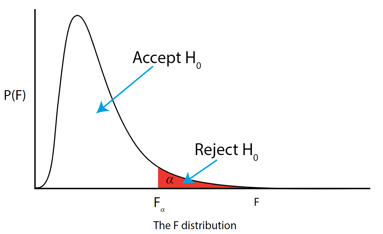
As with all other test statistics, a threshold (critical) value of \(F\) is established. This \(F\) value can be obtained from statistical tables or software and is referred to as \(F_{\text{critical}}\) or \(F_{\alpha}\). As a reminder, this critical value is the minimum value for the test statistic (in this case the F test) for us to be able to reject the null.

The \(F\) distribution, \(F_{\alpha}\), and the location of acceptance and rejection regions are shown in the graph below:

Step 7: Based on steps 5 and 6, draw a conclusion about H0

If the \(F_{\text{\calculated}}\) from the data is larger than the \(F_{\alpha}\), then you are in the rejection region and you can reject the null hypothesis with \((1 - \alpha)\) level of confidence.

Note that modern statistical software condenses steps 6 and 7 by providing a \(p\)-value. The \(p\)-value here is the probability of getting an \(F_{\text{calculated}}\) even greater than what you observe assuming the null hypothesis is true. If by chance, the \(F_{\text{calculated}} = F_{\alpha}\), then the \(p\)-value would exactly equal \(\alpha\). With larger \(F_{\text{calculated}}\) values, we move further into the rejection region and the \(p\) - value becomes less than \(\alpha\). So the decision rule is as follows:

If the \(p\) - value obtained from the ANOVA is less than \(\alpha\), then reject \(H_{0}\) and accept \(H_{A}\).

If you are not familiar with this material, we suggest that you review course materials from your basic statistics course.

Have a language expert improve your writing

Run a free plagiarism check in 10 minutes, generate accurate citations for free.

• Knowledge Base
• Choosing the Right Statistical Test | Types & Examples

Choosing the Right Statistical Test | Types & Examples

Published on January 28, 2020 by Rebecca Bevans . Revised on June 22, 2023.

Statistical tests are used in hypothesis testing . They can be used to:

• determine whether a predictor variable has a statistically significant relationship with an outcome variable.
• estimate the difference between two or more groups.

Statistical tests assume a null hypothesis of no relationship or no difference between groups. Then they determine whether the observed data fall outside of the range of values predicted by the null hypothesis.

If you already know what types of variables you’re dealing with, you can use the flowchart to choose the right statistical test for your data.

Statistical tests flowchart

Table of contents

What does a statistical test do, when to perform a statistical test, choosing a parametric test: regression, comparison, or correlation, choosing a nonparametric test, flowchart: choosing a statistical test, other interesting articles, frequently asked questions about statistical tests.

Statistical tests work by calculating a test statistic – a number that describes how much the relationship between variables in your test differs from the null hypothesis of no relationship.

It then calculates a p value (probability value). The p -value estimates how likely it is that you would see the difference described by the test statistic if the null hypothesis of no relationship were true.

If the value of the test statistic is more extreme than the statistic calculated from the null hypothesis, then you can infer a statistically significant relationship between the predictor and outcome variables.

If the value of the test statistic is less extreme than the one calculated from the null hypothesis, then you can infer no statistically significant relationship between the predictor and outcome variables.

Prevent plagiarism. Run a free check.

You can perform statistical tests on data that have been collected in a statistically valid manner – either through an experiment , or through observations made using probability sampling methods .

For a statistical test to be valid , your sample size needs to be large enough to approximate the true distribution of the population being studied.

To determine which statistical test to use, you need to know:

• whether your data meets certain assumptions.
• the types of variables that you’re dealing with.

Statistical assumptions

Statistical tests make some common assumptions about the data they are testing:

• Independence of observations (a.k.a. no autocorrelation): The observations/variables you include in your test are not related (for example, multiple measurements of a single test subject are not independent, while measurements of multiple different test subjects are independent).
• Homogeneity of variance : the variance within each group being compared is similar among all groups. If one group has much more variation than others, it will limit the test’s effectiveness.
• Normality of data : the data follows a normal distribution (a.k.a. a bell curve). This assumption applies only to quantitative data .

If your data do not meet the assumptions of normality or homogeneity of variance, you may be able to perform a nonparametric statistical test , which allows you to make comparisons without any assumptions about the data distribution.

If your data do not meet the assumption of independence of observations, you may be able to use a test that accounts for structure in your data (repeated-measures tests or tests that include blocking variables).

Types of variables

The types of variables you have usually determine what type of statistical test you can use.

Quantitative variables represent amounts of things (e.g. the number of trees in a forest). Types of quantitative variables include:

• Continuous (aka ratio variables): represent measures and can usually be divided into units smaller than one (e.g. 0.75 grams).
• Discrete (aka integer variables): represent counts and usually can’t be divided into units smaller than one (e.g. 1 tree).

Categorical variables represent groupings of things (e.g. the different tree species in a forest). Types of categorical variables include:

• Ordinal : represent data with an order (e.g. rankings).
• Nominal : represent group names (e.g. brands or species names).
• Binary : represent data with a yes/no or 1/0 outcome (e.g. win or lose).

Choose the test that fits the types of predictor and outcome variables you have collected (if you are doing an experiment , these are the independent and dependent variables ). Consult the tables below to see which test best matches your variables.

Parametric tests usually have stricter requirements than nonparametric tests, and are able to make stronger inferences from the data. They can only be conducted with data that adheres to the common assumptions of statistical tests.

The most common types of parametric test include regression tests, comparison tests, and correlation tests.

Regression tests

Regression tests look for cause-and-effect relationships . They can be used to estimate the effect of one or more continuous variables on another variable.

Comparison tests

Comparison tests look for differences among group means . They can be used to test the effect of a categorical variable on the mean value of some other characteristic.

T-tests are used when comparing the means of precisely two groups (e.g., the average heights of men and women). ANOVA and MANOVA tests are used when comparing the means of more than two groups (e.g., the average heights of children, teenagers, and adults).

Correlation tests

Correlation tests check whether variables are related without hypothesizing a cause-and-effect relationship.

These can be used to test whether two variables you want to use in (for example) a multiple regression test are autocorrelated.

Non-parametric tests don’t make as many assumptions about the data, and are useful when one or more of the common statistical assumptions are violated. However, the inferences they make aren’t as strong as with parametric tests.

This flowchart helps you choose among parametric tests. For nonparametric alternatives, check the table above.

If you want to know more about statistics , methodology , or research bias , make sure to check out some of our other articles with explanations and examples.

• Normal distribution
• Descriptive statistics
• Measures of central tendency
• Correlation coefficient
• Null hypothesis

Methodology

• Cluster sampling
• Stratified sampling
• Types of interviews
• Cohort study
• Thematic analysis

Research bias

• Implicit bias
• Cognitive bias
• Survivorship bias
• Availability heuristic
• Nonresponse bias
• Regression to the mean

Statistical tests commonly assume that:

• the data are normally distributed
• the groups that are being compared have similar variance
• the data are independent

If your data does not meet these assumptions you might still be able to use a nonparametric statistical test , which have fewer requirements but also make weaker inferences.

A test statistic is a number calculated by a  statistical test . It describes how far your observed data is from the  null hypothesis  of no relationship between  variables or no difference among sample groups.

The test statistic tells you how different two or more groups are from the overall population mean , or how different a linear slope is from the slope predicted by a null hypothesis . Different test statistics are used in different statistical tests.

Statistical significance is a term used by researchers to state that it is unlikely their observations could have occurred under the null hypothesis of a statistical test . Significance is usually denoted by a p -value , or probability value.

Statistical significance is arbitrary – it depends on the threshold, or alpha value, chosen by the researcher. The most common threshold is p < 0.05, which means that the data is likely to occur less than 5% of the time under the null hypothesis .

When the p -value falls below the chosen alpha value, then we say the result of the test is statistically significant.

Quantitative variables are any variables where the data represent amounts (e.g. height, weight, or age).

Categorical variables are any variables where the data represent groups. This includes rankings (e.g. finishing places in a race), classifications (e.g. brands of cereal), and binary outcomes (e.g. coin flips).

You need to know what type of variables you are working with to choose the right statistical test for your data and interpret your results .

Discrete and continuous variables are two types of quantitative variables :

• Discrete variables represent counts (e.g. the number of objects in a collection).
• Continuous variables represent measurable amounts (e.g. water volume or weight).

Cite this Scribbr article

If you want to cite this source, you can copy and paste the citation or click the “Cite this Scribbr article” button to automatically add the citation to our free Citation Generator.

Bevans, R. (2023, June 22). Choosing the Right Statistical Test | Types & Examples. Scribbr. Retrieved April 2, 2024, from https://www.scribbr.com/statistics/statistical-tests/

Is this article helpful?

Rebecca Bevans

Other students also liked, hypothesis testing | a step-by-step guide with easy examples, test statistics | definition, interpretation, and examples, normal distribution | examples, formulas, & uses, what is your plagiarism score.

9.1 Null and Alternative Hypotheses

The actual test begins by considering two hypotheses . They are called the null hypothesis and the alternative hypothesis . These hypotheses contain opposing viewpoints.

H 0 , the — null hypothesis: a statement of no difference between sample means or proportions or no difference between a sample mean or proportion and a population mean or proportion. In other words, the difference equals 0.

H a —, the alternative hypothesis: a claim about the population that is contradictory to H 0 and what we conclude when we reject H 0 .

Since the null and alternative hypotheses are contradictory, you must examine evidence to decide if you have enough evidence to reject the null hypothesis or not. The evidence is in the form of sample data.

After you have determined which hypothesis the sample supports, you make a decision. There are two options for a decision. They are reject H 0 if the sample information favors the alternative hypothesis or do not reject H 0 or decline to reject H 0 if the sample information is insufficient to reject the null hypothesis.

Mathematical Symbols Used in H 0 and H a :

H 0 always has a symbol with an equal in it. H a never has a symbol with an equal in it. The choice of symbol depends on the wording of the hypothesis test. However, be aware that many researchers use = in the null hypothesis, even with > or < as the symbol in the alternative hypothesis. This practice is acceptable because we only make the decision to reject or not reject the null hypothesis.

Example 9.1

H 0 : No more than 30 percent of the registered voters in Santa Clara County voted in the primary election. p ≤ 30 H a : More than 30 percent of the registered voters in Santa Clara County voted in the primary election. p > 30

A medical trial is conducted to test whether or not a new medicine reduces cholesterol by 25 percent. State the null and alternative hypotheses.

Example 9.2

We want to test whether the mean GPA of students in American colleges is different from 2.0 (out of 4.0). The null and alternative hypotheses are the following: H 0 : μ = 2.0 H a : μ ≠ 2.0

We want to test whether the mean height of eighth graders is 66 inches. State the null and alternative hypotheses. Fill in the correct symbol (=, ≠, ≥, <, ≤, >) for the null and alternative hypotheses.

• H 0 : μ __ 66
• H a : μ __ 66

Example 9.3

We want to test if college students take fewer than five years to graduate from college, on the average. The null and alternative hypotheses are the following: H 0 : μ ≥ 5 H a : μ < 5

We want to test if it takes fewer than 45 minutes to teach a lesson plan. State the null and alternative hypotheses. Fill in the correct symbol ( =, ≠, ≥, <, ≤, >) for the null and alternative hypotheses.

• H 0 : μ __ 45
• H a : μ __ 45

Example 9.4

An article on school standards stated that about half of all students in France, Germany, and Israel take advanced placement exams and a third of the students pass. The same article stated that 6.6 percent of U.S. students take advanced placement exams and 4.4 percent pass. Test if the percentage of U.S. students who take advanced placement exams is more than 6.6 percent. State the null and alternative hypotheses. H 0 : p ≤ 0.066 H a : p > 0.066

On a state driver’s test, about 40 percent pass the test on the first try. We want to test if more than 40 percent pass on the first try. Fill in the correct symbol (=, ≠, ≥, <, ≤, >) for the null and alternative hypotheses.

• H 0 : p __ 0.40
• H a : p __ 0.40

Collaborative Exercise

Bring to class a newspaper, some news magazines, and some internet articles. In groups, find articles from which your group can write null and alternative hypotheses. Discuss your hypotheses with the rest of the class.

As an Amazon Associate we earn from qualifying purchases.

This book may not be used in the training of large language models or otherwise be ingested into large language models or generative AI offerings without OpenStax's permission.

Want to cite, share, or modify this book? This book uses the Creative Commons Attribution License and you must attribute Texas Education Agency (TEA). The original material is available at: https://www.texasgateway.org/book/tea-statistics . Changes were made to the original material, including updates to art, structure, and other content updates.

Access for free at https://openstax.org/books/statistics/pages/1-introduction

• Authors: Barbara Illowsky, Susan Dean
• Publisher/website: OpenStax
• Book title: Statistics
• Publication date: Mar 27, 2020
• Location: Houston, Texas
• Book URL: https://openstax.org/books/statistics/pages/1-introduction
• Section URL: https://openstax.org/books/statistics/pages/9-1-null-and-alternative-hypotheses

© Jan 23, 2024 Texas Education Agency (TEA). The OpenStax name, OpenStax logo, OpenStax book covers, OpenStax CNX name, and OpenStax CNX logo are not subject to the Creative Commons license and may not be reproduced without the prior and express written consent of Rice University.

Hypothesis Testing

Hypothesis testing is a tool for making statistical inferences about the population data. It is an analysis tool that tests assumptions and determines how likely something is within a given standard of accuracy. Hypothesis testing provides a way to verify whether the results of an experiment are valid.

A null hypothesis and an alternative hypothesis are set up before performing the hypothesis testing. This helps to arrive at a conclusion regarding the sample obtained from the population. In this article, we will learn more about hypothesis testing, its types, steps to perform the testing, and associated examples.

What is Hypothesis Testing in Statistics?

Hypothesis testing uses sample data from the population to draw useful conclusions regarding the population probability distribution . It tests an assumption made about the data using different types of hypothesis testing methodologies. The hypothesis testing results in either rejecting or not rejecting the null hypothesis.

Hypothesis Testing Definition

Hypothesis testing can be defined as a statistical tool that is used to identify if the results of an experiment are meaningful or not. It involves setting up a null hypothesis and an alternative hypothesis. These two hypotheses will always be mutually exclusive. This means that if the null hypothesis is true then the alternative hypothesis is false and vice versa. An example of hypothesis testing is setting up a test to check if a new medicine works on a disease in a more efficient manner.

Null Hypothesis

The null hypothesis is a concise mathematical statement that is used to indicate that there is no difference between two possibilities. In other words, there is no difference between certain characteristics of data. This hypothesis assumes that the outcomes of an experiment are based on chance alone. It is denoted as \(H_{0}\). Hypothesis testing is used to conclude if the null hypothesis can be rejected or not. Suppose an experiment is conducted to check if girls are shorter than boys at the age of 5. The null hypothesis will say that they are the same height.

Alternative Hypothesis

The alternative hypothesis is an alternative to the null hypothesis. It is used to show that the observations of an experiment are due to some real effect. It indicates that there is a statistical significance between two possible outcomes and can be denoted as \(H_{1}\) or \(H_{a}\). For the above-mentioned example, the alternative hypothesis would be that girls are shorter than boys at the age of 5.

Hypothesis Testing P Value

In hypothesis testing, the p value is used to indicate whether the results obtained after conducting a test are statistically significant or not. It also indicates the probability of making an error in rejecting or not rejecting the null hypothesis.This value is always a number between 0 and 1. The p value is compared to an alpha level, \(\alpha\) or significance level. The alpha level can be defined as the acceptable risk of incorrectly rejecting the null hypothesis. The alpha level is usually chosen between 1% to 5%.

Hypothesis Testing Critical region

All sets of values that lead to rejecting the null hypothesis lie in the critical region. Furthermore, the value that separates the critical region from the non-critical region is known as the critical value.

Hypothesis Testing Formula

Depending upon the type of data available and the size, different types of hypothesis testing are used to determine whether the null hypothesis can be rejected or not. The hypothesis testing formula for some important test statistics are given below:

• z = \(\frac{\overline{x}-\mu}{\frac{\sigma}{\sqrt{n}}}\). \(\overline{x}\) is the sample mean, \(\mu\) is the population mean, \(\sigma\) is the population standard deviation and n is the size of the sample.
• t = \(\frac{\overline{x}-\mu}{\frac{s}{\sqrt{n}}}\). s is the sample standard deviation.
• \(\chi ^{2} = \sum \frac{(O_{i}-E_{i})^{2}}{E_{i}}\). \(O_{i}\) is the observed value and \(E_{i}\) is the expected value.

We will learn more about these test statistics in the upcoming section.

Types of Hypothesis Testing

Selecting the correct test for performing hypothesis testing can be confusing. These tests are used to determine a test statistic on the basis of which the null hypothesis can either be rejected or not rejected. Some of the important tests used for hypothesis testing are given below.

Hypothesis Testing Z Test

A z test is a way of hypothesis testing that is used for a large sample size (n ≥ 30). It is used to determine whether there is a difference between the population mean and the sample mean when the population standard deviation is known. It can also be used to compare the mean of two samples. It is used to compute the z test statistic. The formulas are given as follows:

• One sample: z = \(\frac{\overline{x}-\mu}{\frac{\sigma}{\sqrt{n}}}\).
• Two samples: z = \(\frac{(\overline{x_{1}}-\overline{x_{2}})-(\mu_{1}-\mu_{2})}{\sqrt{\frac{\sigma_{1}^{2}}{n_{1}}+\frac{\sigma_{2}^{2}}{n_{2}}}}\).

Hypothesis Testing t Test

The t test is another method of hypothesis testing that is used for a small sample size (n < 30). It is also used to compare the sample mean and population mean. However, the population standard deviation is not known. Instead, the sample standard deviation is known. The mean of two samples can also be compared using the t test.

• One sample: t = \(\frac{\overline{x}-\mu}{\frac{s}{\sqrt{n}}}\).
• Two samples: t = \(\frac{(\overline{x_{1}}-\overline{x_{2}})-(\mu_{1}-\mu_{2})}{\sqrt{\frac{s_{1}^{2}}{n_{1}}+\frac{s_{2}^{2}}{n_{2}}}}\).

Hypothesis Testing Chi Square

The Chi square test is a hypothesis testing method that is used to check whether the variables in a population are independent or not. It is used when the test statistic is chi-squared distributed.

One Tailed Hypothesis Testing

One tailed hypothesis testing is done when the rejection region is only in one direction. It can also be known as directional hypothesis testing because the effects can be tested in one direction only. This type of testing is further classified into the right tailed test and left tailed test.

Right Tailed Hypothesis Testing

The right tail test is also known as the upper tail test. This test is used to check whether the population parameter is greater than some value. The null and alternative hypotheses for this test are given as follows:

\(H_{0}\): The population parameter is ≤ some value

\(H_{1}\): The population parameter is > some value.

If the test statistic has a greater value than the critical value then the null hypothesis is rejected

Left Tailed Hypothesis Testing

The left tail test is also known as the lower tail test. It is used to check whether the population parameter is less than some value. The hypotheses for this hypothesis testing can be written as follows:

\(H_{0}\): The population parameter is ≥ some value

\(H_{1}\): The population parameter is < some value.

The null hypothesis is rejected if the test statistic has a value lesser than the critical value.

Two Tailed Hypothesis Testing

In this hypothesis testing method, the critical region lies on both sides of the sampling distribution. It is also known as a non - directional hypothesis testing method. The two-tailed test is used when it needs to be determined if the population parameter is assumed to be different than some value. The hypotheses can be set up as follows:

\(H_{0}\): the population parameter = some value

\(H_{1}\): the population parameter ≠ some value

The null hypothesis is rejected if the test statistic has a value that is not equal to the critical value.

Hypothesis Testing Steps

Hypothesis testing can be easily performed in five simple steps. The most important step is to correctly set up the hypotheses and identify the right method for hypothesis testing. The basic steps to perform hypothesis testing are as follows:

• Step 1: Set up the null hypothesis by correctly identifying whether it is the left-tailed, right-tailed, or two-tailed hypothesis testing.
• Step 2: Set up the alternative hypothesis.
• Step 3: Choose the correct significance level, \(\alpha\), and find the critical value.
• Step 4: Calculate the correct test statistic (z, t or \(\chi\)) and p-value.
• Step 5: Compare the test statistic with the critical value or compare the p-value with \(\alpha\) to arrive at a conclusion. In other words, decide if the null hypothesis is to be rejected or not.

Hypothesis Testing Example

The best way to solve a problem on hypothesis testing is by applying the 5 steps mentioned in the previous section. Suppose a researcher claims that the mean average weight of men is greater than 100kgs with a standard deviation of 15kgs. 30 men are chosen with an average weight of 112.5 Kgs. Using hypothesis testing, check if there is enough evidence to support the researcher's claim. The confidence interval is given as 95%.

Step 1: This is an example of a right-tailed test. Set up the null hypothesis as \(H_{0}\): \(\mu\) = 100.

Step 2: The alternative hypothesis is given by \(H_{1}\): \(\mu\) > 100.

Step 3: As this is a one-tailed test, \(\alpha\) = 100% - 95% = 5%. This can be used to determine the critical value.

1 - \(\alpha\) = 1 - 0.05 = 0.95

0.95 gives the required area under the curve. Now using a normal distribution table, the area 0.95 is at z = 1.645. A similar process can be followed for a t-test. The only additional requirement is to calculate the degrees of freedom given by n - 1.

Step 4: Calculate the z test statistic. This is because the sample size is 30. Furthermore, the sample and population means are known along with the standard deviation.

z = \(\frac{\overline{x}-\mu}{\frac{\sigma}{\sqrt{n}}}\).

\(\mu\) = 100, \(\overline{x}\) = 112.5, n = 30, \(\sigma\) = 15

z = \(\frac{112.5-100}{\frac{15}{\sqrt{30}}}\) = 4.56

Step 5: Conclusion. As 4.56 > 1.645 thus, the null hypothesis can be rejected.

Hypothesis Testing and Confidence Intervals

Confidence intervals form an important part of hypothesis testing. This is because the alpha level can be determined from a given confidence interval. Suppose a confidence interval is given as 95%. Subtract the confidence interval from 100%. This gives 100 - 95 = 5% or 0.05. This is the alpha value of a one-tailed hypothesis testing. To obtain the alpha value for a two-tailed hypothesis testing, divide this value by 2. This gives 0.05 / 2 = 0.025.

Related Articles:

• Probability and Statistics
• Data Handling

Important Notes on Hypothesis Testing

• Hypothesis testing is a technique that is used to verify whether the results of an experiment are statistically significant.
• It involves the setting up of a null hypothesis and an alternate hypothesis.
• There are three types of tests that can be conducted under hypothesis testing - z test, t test, and chi square test.
• Hypothesis testing can be classified as right tail, left tail, and two tail tests.

Examples on Hypothesis Testing

• Example 1: The average weight of a dumbbell in a gym is 90lbs. However, a physical trainer believes that the average weight might be higher. A random sample of 5 dumbbells with an average weight of 110lbs and a standard deviation of 18lbs. Using hypothesis testing check if the physical trainer's claim can be supported for a 95% confidence level. Solution: As the sample size is lesser than 30, the t-test is used. \(H_{0}\): \(\mu\) = 90, \(H_{1}\): \(\mu\) > 90 \(\overline{x}\) = 110, \(\mu\) = 90, n = 5, s = 18. \(\alpha\) = 0.05 Using the t-distribution table, the critical value is 2.132 t = \(\frac{\overline{x}-\mu}{\frac{s}{\sqrt{n}}}\) t = 2.484 As 2.484 > 2.132, the null hypothesis is rejected. Answer: The average weight of the dumbbells may be greater than 90lbs
• Example 2: The average score on a test is 80 with a standard deviation of 10. With a new teaching curriculum introduced it is believed that this score will change. On random testing, the score of 38 students, the mean was found to be 88. With a 0.05 significance level, is there any evidence to support this claim? Solution: This is an example of two-tail hypothesis testing. The z test will be used. \(H_{0}\): \(\mu\) = 80, \(H_{1}\): \(\mu\) ≠ 80 \(\overline{x}\) = 88, \(\mu\) = 80, n = 36, \(\sigma\) = 10. \(\alpha\) = 0.05 / 2 = 0.025 The critical value using the normal distribution table is 1.96 z = \(\frac{\overline{x}-\mu}{\frac{\sigma}{\sqrt{n}}}\) z = \(\frac{88-80}{\frac{10}{\sqrt{36}}}\) = 4.8 As 4.8 > 1.96, the null hypothesis is rejected. Answer: There is a difference in the scores after the new curriculum was introduced.
• Example 3: The average score of a class is 90. However, a teacher believes that the average score might be lower. The scores of 6 students were randomly measured. The mean was 82 with a standard deviation of 18. With a 0.05 significance level use hypothesis testing to check if this claim is true. Solution: The t test will be used. \(H_{0}\): \(\mu\) = 90, \(H_{1}\): \(\mu\) < 90 \(\overline{x}\) = 110, \(\mu\) = 90, n = 6, s = 18 The critical value from the t table is -2.015 t = \(\frac{\overline{x}-\mu}{\frac{s}{\sqrt{n}}}\) t = \(\frac{82-90}{\frac{18}{\sqrt{6}}}\) t = -1.088 As -1.088 > -2.015, we fail to reject the null hypothesis. Answer: There is not enough evidence to support the claim.

go to slide go to slide go to slide

Book a Free Trial Class

FAQs on Hypothesis Testing

What is hypothesis testing.

Hypothesis testing in statistics is a tool that is used to make inferences about the population data. It is also used to check if the results of an experiment are valid.

What is the z Test in Hypothesis Testing?

The z test in hypothesis testing is used to find the z test statistic for normally distributed data . The z test is used when the standard deviation of the population is known and the sample size is greater than or equal to 30.

What is the t Test in Hypothesis Testing?

The t test in hypothesis testing is used when the data follows a student t distribution . It is used when the sample size is less than 30 and standard deviation of the population is not known.

What is the formula for z test in Hypothesis Testing?

The formula for a one sample z test in hypothesis testing is z = \(\frac{\overline{x}-\mu}{\frac{\sigma}{\sqrt{n}}}\) and for two samples is z = \(\frac{(\overline{x_{1}}-\overline{x_{2}})-(\mu_{1}-\mu_{2})}{\sqrt{\frac{\sigma_{1}^{2}}{n_{1}}+\frac{\sigma_{2}^{2}}{n_{2}}}}\).

What is the p Value in Hypothesis Testing?

The p value helps to determine if the test results are statistically significant or not. In hypothesis testing, the null hypothesis can either be rejected or not rejected based on the comparison between the p value and the alpha level.

What is One Tail Hypothesis Testing?

When the rejection region is only on one side of the distribution curve then it is known as one tail hypothesis testing. The right tail test and the left tail test are two types of directional hypothesis testing.

What is the Alpha Level in Two Tail Hypothesis Testing?

To get the alpha level in a two tail hypothesis testing divide \(\alpha\) by 2. This is done as there are two rejection regions in the curve.

Statistics Tutorial

Descriptive statistics, inferential statistics, stat reference, statistics - hypothesis testing.

Hypothesis testing is a formal way of checking if a hypothesis about a population is true or not.

Hypothesis Testing

A hypothesis is a claim about a population parameter .

A hypothesis test is a formal procedure to check if a hypothesis is true or not.

Examples of claims that can be checked:

The average height of people in Denmark is more than 170 cm.

The share of left handed people in Australia is not 10%.

The average income of dentists is less the average income of lawyers.

The Null and Alternative Hypothesis

Hypothesis testing is based on making two different claims about a population parameter.

The null hypothesis (\(H_{0} \)) and the alternative hypothesis (\(H_{1}\)) are the claims.

The two claims needs to be mutually exclusive , meaning only one of them can be true.

The alternative hypothesis is typically what we are trying to prove.

For example, we want to check the following claim:

"The average height of people in Denmark is more than 170 cm."

In this case, the parameter is the average height of people in Denmark (\(\mu\)).

The null and alternative hypothesis would be:

Null hypothesis : The average height of people in Denmark is 170 cm.

Alternative hypothesis : The average height of people in Denmark is more than 170 cm.

The claims are often expressed with symbols like this:

\(H_{0}\): \(\mu = 170 \: cm \)

\(H_{1}\): \(\mu > 170 \: cm \)

If the data supports the alternative hypothesis, we reject the null hypothesis and accept the alternative hypothesis.

If the data does not support the alternative hypothesis, we keep the null hypothesis.

Note: The alternative hypothesis is also referred to as (\(H_{A} \)).

The Significance Level

The significance level (\(\alpha\)) is the uncertainty we accept when rejecting the null hypothesis in the hypothesis test.

The significance level is a percentage probability of accidentally making the wrong conclusion.

Typical significance levels are:

• \(\alpha = 0.1\) (10%)
• \(\alpha = 0.05\) (5%)
• \(\alpha = 0.01\) (1%)

A lower significance level means that the evidence in the data needs to be stronger to reject the null hypothesis.

There is no "correct" significance level - it only states the uncertainty of the conclusion.

Note: A 5% significance level means that when we reject a null hypothesis:

We expect to reject a true null hypothesis 5 out of 100 times.

Advertisement

The Test Statistic

The test statistic is used to decide the outcome of the hypothesis test.

The test statistic is a standardized value calculated from the sample.

Standardization means converting a statistic to a well known probability distribution .

The type of probability distribution depends on the type of test.

Common examples are:

• Standard Normal Distribution (Z): used for Testing Population Proportions
• Student's T-Distribution (T): used for Testing Population Means

Note: You will learn how to calculate the test statistic for each type of test in the following chapters.

The Critical Value and P-Value Approach

There are two main approaches used for hypothesis tests:

• The critical value approach compares the test statistic with the critical value of the significance level.
• The p-value approach compares the p-value of the test statistic and with the significance level.

The Critical Value Approach

The critical value approach checks if the test statistic is in the rejection region .

The rejection region is an area of probability in the tails of the distribution.

The size of the rejection region is decided by the significance level (\(\alpha\)).

The value that separates the rejection region from the rest is called the critical value .

Here is a graphical illustration:

If the test statistic is inside this rejection region, the null hypothesis is rejected .

For example, if the test statistic is 2.3 and the critical value is 2 for a significance level (\(\alpha = 0.05\)):

We reject the null hypothesis (\(H_{0} \)) at 0.05 significance level (\(\alpha\))

The P-Value Approach

The p-value approach checks if the p-value of the test statistic is smaller than the significance level (\(\alpha\)).

The p-value of the test statistic is the area of probability in the tails of the distribution from the value of the test statistic.

If the p-value is smaller than the significance level, the null hypothesis is rejected .

The p-value directly tells us the lowest significance level where we can reject the null hypothesis.

For example, if the p-value is 0.03:

We reject the null hypothesis (\(H_{0} \)) at a 0.05 significance level (\(\alpha\))

We keep the null hypothesis (\(H_{0}\)) at a 0.01 significance level (\(\alpha\))

Note: The two approaches are only different in how they present the conclusion.

Steps for a Hypothesis Test

The following steps are used for a hypothesis test:

• Check the conditions
• Define the claims
• Decide the significance level
• Calculate the test statistic

One condition is that the sample is randomly selected from the population.

The other conditions depends on what type of parameter you are testing the hypothesis for.

Common parameters to test hypotheses are:

• Proportions (for qualitative data)
• Mean values (for numerical data)

You will learn the steps for both types in the following pages.

COLOR PICKER

Report Error

If you want to report an error, or if you want to make a suggestion, do not hesitate to send us an e-mail:

[email protected]

Top Tutorials

Top references, top examples, get certified.

Confidence distributions and hypothesis testing

• Regular Article
• Open access
• Published: 29 March 2024

Cite this article

You have full access to this open access article

• Eugenio Melilli   ORCID: orcid.org/0000-0003-2542-5286 1 &
• Piero Veronese   ORCID: orcid.org/0000-0002-4416-2269 1  

68 Accesses

Explore all metrics

The traditional frequentist approach to hypothesis testing has recently come under extensive debate, raising several critical concerns. Additionally, practical applications often blend the decision-theoretical framework pioneered by Neyman and Pearson with the inductive inferential process relied on the p -value, as advocated by Fisher. The combination of the two methods has led to interpreting the p -value as both an observed error rate and a measure of empirical evidence for the hypothesis. Unfortunately, both interpretations pose difficulties. In this context, we propose that resorting to confidence distributions can offer a valuable solution to address many of these critical issues. Rather than suggesting an automatic procedure, we present a natural approach to tackle the problem within a broader inferential context. Through the use of confidence distributions, we show the possibility of defining two statistical measures of evidence that align with different types of hypotheses under examination. These measures, unlike the p -value, exhibit coherence, simplicity of interpretation, and ease of computation, as exemplified by various illustrative examples spanning diverse fields. Furthermore, we provide theoretical results that establish connections between our proposal, other measures of evidence given in the literature, and standard testing concepts such as size, optimality, and the p -value.

Similar content being viewed by others

Blending bayesian and frequentist methods according to the precision of prior information with applications to hypothesis testing.

David R. Bickel

Introducing and analyzing the Bayesian power function as an alternative to the power function for a test

Julián de la Horra

The Support Interval

Eric-Jan Wagenmakers, Quentin F. Gronau, … Alexander Etz

Avoid common mistakes on your manuscript.

1 Introduction

In applied research, the standard frequentist approach to hypothesis testing is commonly regarded as a straightforward, coherent, and automatic method for assessing the validity of a conjecture represented by one of two hypotheses, denoted as \({{{\mathcal {H}}}_{0}}\) and \({{{\mathcal {H}}}_{1}}\) . The probabilities \(\alpha \) and \(\beta \) of committing type I and type II errors (reject \({{{\mathcal {H}}}_{0}}\) , when it is true and accept \({{{\mathcal {H}}}_{0}}\) when it is false, respectively) are controlled through a carefully designed experiment. After having fixed \(\alpha \) (usually at 0.05), the p -value is used to quantify the measure of evidence against the null hypothesis. If the p -value is less than \(\alpha \) , the conclusion is deemed significant , suggesting that it is unlikely that the null hypothesis holds. Regrettably, this methodology is not as secure as it may seem, as evidenced by a large literature, see the ASA’s Statement on p -values (Wasserstein and Lazar 2016 ) and The American Statistician (2019, vol. 73, sup1) for a discussion of various principles, misconceptions, and recommendations regarding the utilization of p -values. The standard frequentist approach is, in fact, a blend of two different views on hypothesis testing presented by Neyman-Pearson and Fisher. The first authors approach hypothesis testing within a decision-theoretic framework, viewing it as a behavioral theory. In contrast, Fisher’s perspective considers testing as a component of an inductive inferential process that does not necessarily require an alternative hypothesis or concepts from decision theory such as loss, risk or admissibility, see Hubbard and Bayarri ( 2003 ). As emphasized by Goodman ( 1993 ) “the combination of the two methods has led to a reinterpretation of the p -value simultaneously as an ‘observed error rate’ and as a ‘measure of evidence’. Both of these interpretations are problematic...”.

It is out of our scope to review the extensive debate on hypothesis testing. Here, we briefly touch upon a few general points, without delving into the Bayesian approach.

i) The long-standing caution expressed by Berger and Sellke ( 1987 ) and Berger and Delampady ( 1987 ) that a p -value of 0.05 provides only weak evidence against the null hypothesis has been further substantiated by recent investigations into experiment reproducibility, see e.g., Open Science Collaboration OSC ( 2015 ) and Johnson et al. ( 2017 ). In light of this, 72 statisticians have stated “For fields where the threshold for defining statistical significance for new discoveries is \(p<0.05\) , we propose a change to \(p<0.005\) ”, see Benjamin et al. ( 2018 ).

ii) The ongoing debate regarding the selection of a one-sided or two-sided test leaves the standard practice of doubling the p-value , when moving from the first to the second type of test, without consistent support, see e.g., Freedman ( 2008 ).

iii) There has been a longstanding argument in favor of integrating hypothesis testing with estimation, see e.g. Yates ( 1951 , pp. 32–33) or more recently, Greenland et al. ( 2016 ) who emphasize that “... statistical tests should never constitute the sole input to inferences or decisions about associations or effects ... in most scientific settings, the arbitrary classification of results into significant and non-significant is unnecessary for and often damaging to valid interpretation of data”.

iv) Finally, the p -value is incoherent when it is regarded as a statistical measure of the evidence provided by the data in support of a hypothesis \({{{\mathcal {H}}}_{0}}\) . As shown by Schervish ( 1996 ), it is possible that the p -value for testing the hypothesis \({{{\mathcal {H}}}_{0}}\) is greater than that for testing \({{{\mathcal {H}}}_{0}}^{\prime } \supset {{{\mathcal {H}}}_{0}}\) for the same observed data.

While theoretical insights into hypothesis testing are valuable for elucidating various aspects, we believe they cannot be compelled to serve as a unique, definitive practical guide for real-world applications. For example, uniformly most powerful (UMP) tests for discrete models not only rarely exist, but nobody uses them because they are randomized. On the other hand, how can a test of size 0.05 be considered really different from one of size 0.047 or 0.053? Moreover, for one-sided hypotheses, why should the first type error always be much more severe than the second type one? Alternatively, why should the test for \({{{\mathcal {H}}}_{0}}: \theta \le \theta _0\) versus \({{{\mathcal {H}}}_{1}}: \theta >\theta _0\) always be considered equivalent to the test for \({{{\mathcal {H}}}_{0}}: \theta = \theta _0\) versus \({{{\mathcal {H}}}_{1}}: \theta >\theta _0\) ? Furthermore, the decision to test \({{{\mathcal {H}}}_{0}}: \theta =\theta _0\) rather than \({{{\mathcal {H}}}_{0}}: \theta \in [\theta _0-\epsilon , \theta _0+\epsilon ]\) , for a suitable positive \(\epsilon \) , should be driven by the specific requirements of the application and not solely by the existence of a good or simple test. In summary, we concur with Fisher ( 1973 ) that “no scientific worker has a fixed level of significance at which from year to year, and in all circumstances, he rejects hypotheses; he rather gives his mind to each particular case in the light of his evidence and his ideas”.

Considering all these crucial aspects, we believe it is essential to seek an applied hypothesis testing approach that encourages researchers to engage more deeply with the specific problem, avoids relying on standardized procedures, and is consistently integrated into a broader framework of inference. One potential solution can be found resorting to the “confidence distribution” (CD) approach. The modern CD theory was introduced by Schweder and Hjort ( 2002 ) and Singh et al. ( 2005 ) and relies on the idea of constructing a data-depending distribution for the parameter of interest to be used for inferential purposes. A CD should not be confused with a Bayesian posterior distribution. It is not derived through the Bayes theorem, and it does not require any prior distributions. Similar to the conventional practice in point or interval estimation, where one seeks a point or interval estimator, the objective of this theory is to discover a distribution estimator . Thanks to a clarification of this concept and a formalized definition of the CD within a purely frequentist setting, a wide literature on the topic has been developed encompassing both theoretical developments and practical applications, see e.g. for a general overview Schweder and Hjort ( 2016 ), Singh et al. ( 2007 ), and Xie and Singh ( 2013 ). We also remark that when inference is required for a real parameter, it is possible to establish a relationship between CDs and fiducial distributions, originally introduced by Fisher ( 1930 ). For a modern and general presentation of the fiducial inference see Hannig ( 2009 ) and Hannig et al. ( 2016 ), while for a connection with the CDs see Schweder and Hjort ( 2016 ) and Veronese and Melilli ( 2015 , 2018a ). Some results about the connection between CDs and hypothesis testing are presented in Singh et al. ( 2007 , Sec. 3.3) and Xie & Singh ( 2013 , Sec. 4.3), but the focus is only on the formal relationships between the support that a CD can provide for a hypothesis and the p -value.

In this paper we discuss in details the application of CDs in hypothesis testing. We show how CDs can offer valuable solutions to address the aforementioned difficulties and how a test can naturally be viewed as a part of a more extensive inferential process. Once a CD has been specified, everything can be developed straightforwardly, without any particular technical difficulties. The core of our approach centers on the notion of support provided by the data to a hypothesis through a CD. We introduce two distinct but related types of support, the choice of which depends on the hypothesis under consideration. They are always coherent, easy to interpret and to compute, even in case of interval hypotheses, contrary to what happens for the p -value. The flexibility, simplicity, and effectiveness of our proposal are illustrated by several examples from various fields and a simulation study. We have postponed the presentation of theoretical results, comparisons with other proposals found in the literature, as well as the connections with standard hypothesis testing concepts such as size, significance level, optimality, and p -values to the end of the paper to enhance its readability.

The paper is structured as follows: In Sect. 2 , we provide a review of the CD’s definition and the primary methods for its construction, with a particular focus on distinctive aspects that arise when dealing with discrete models (Sect. 2.1 ). Section 3 explores the application of the CD in hypothesis testing and introduces the two notions of support. In Sect. 4 , we discuss several examples to illustrate the benefits of utilizing the CD in various scenarios, offering comparisons with traditional p -values. Theoretical results about tests based on the CD and comparisons with other measures of support or plausibility for hypotheses are presented in Sect. 5 . Finally, in Sect. 6 , we summarize the paper’s findings and provide concluding remarks. For convenience, a table of CDs for some common statistical models can be found in Appendix A, while all the proofs of the propositions are presented in Appendix B.

2 Confidence distributions

The modern definition of confidence distribution for a real parameter \(\theta \) of interest, see Schweder & Hjort ( 2002 ; 2016 , sec. 3.2) and Singh et al. ( 2005 ; 2007 ) can be formulated as follows:

Definition 1

Let \(\{P_{\theta ,\varvec{\lambda }},\theta \in \Theta \subseteq \mathbb {R}, \varvec{\lambda }\in \varvec{\Lambda }\}\) be a parametric model for data \(\textbf{X}\in {\mathcal {X}}\) ; here \(\theta \) is the parameter of interest and \(\varvec{\lambda }\) is a nuisance parameter. A function H of \(\textbf{X}\) and \(\theta \) is called a confidence distribution for \(\theta \) if: i) for each value \(\textbf{x}\) of \(\textbf{X}\) , \(H(\textbf{x},\cdot )=H_{\textbf{x}}(\cdot )\) is a continuous distribution function on \(\Theta \) ; ii) \(H(\textbf{X},\theta )\) , seen as a function of the random element \(\textbf{X}\) , has the uniform distribution on (0, 1), whatever the true parameter value \((\theta , \varvec{\lambda })\) . The function H is an asymptotic confidence distribution if the continuity requirement in i) is removed and ii) is replaced by: ii) \(^{\prime }\) \(H(\textbf{X},\theta )\) converges in law to the uniform distribution on (0, 1) for the sample size going to infinity, whatever the true parameter value \((\theta , \varvec{\lambda })\) .

The CD theory is placed in a purely frequentist context and the uniformity of the distribution ensures the correct coverage of the confidence intervals. The CD should be regarded as a distribution estimator of a parameter \(\theta \) and its mean, median or mode can serve as point estimates of \(\theta \) , see Xie and Singh ( 2013 ) for a detailed discussion. In essence, the CD can be employed in a manner similar to a Bayesian posterior distribution, but its interpretation differs and does not necessitate any prior distribution. Closely related to the CD is the confidence curve (CC) which, given an observation \(\textbf{x}\) , is defined as \( CC_{\textbf{x}}(\theta )=|1-2H_{\textbf{x}}(\theta )|\) ; see Schweder and Hjort ( 2002 ). This function provides the boundary points of equal-tailed confidence intervals for any level \(1-\alpha \) , with \(0<\alpha <1\) , and offers an immediate visualization of their length.

Various procedures can be adopted to obtain exact or asymptotic CDs starting, for example, from pivotal functions, likelihood functions and bootstrap distributions, as detailed in Singh et al. ( 2007 ), Xie and Singh ( 2013 ), Schweder and Hjort ( 2016 ). A CD (or an asymptotic CD) can also be derived directly from a real statistic T , provided that its exact or asymptotic distribution function \(F_{\theta }(t)\) is a continuously monotonic function in \(\theta \) and its limits are 0 and 1 as \(\theta \) approaches its boundaries. For example, if \(F_{\theta }(t)\) is nonincreasing, we can define

Furthermore, if \(H_t(\theta )\) is differentiable in \(\theta \) , we can obtain the CD-density \(h_t(\theta )=-({\partial }/{\partial \theta }) F_{\theta }(t)\) , which coincides with the fiducial density suggested by Fisher. In particular, when the statistical model belongs to the real regular natural exponential family (NEF) with natural parameter \(\theta \) and sufficient statistic T , there always exists an “optimal” CD for \(\theta \) which is given by ( 1 ), see Veronese and Melilli ( 2015 ).

The CDs based on a real statistic play an important role in hypothesis testing. In this setting remarkable results are obtained when the model has monotone likelihood ratio (MLR). We recall that if \(\textbf{X}\) is a random vector distributed according to the family \(\{p_\theta , \theta \in \Theta \subseteq \mathbb {R}\}\) , this family is said to have MLR in the real statistic \(T(\textbf{X})\) if, for any \(\theta _1 <\theta _2\) , the ratio \(p_{\theta _2}(\textbf{x})/p_{\theta _1}(\textbf{x})\) is a nondecreasing function of \(T(\textbf{x})\) for values of \(\textbf{x}\) that induce at least one of \(p_{\theta _1}\) and \(p_{\theta _2}\) to be positive. Furthermore, for such families, it holds that \(F_{\theta _2}(t) \le F_{\theta _1}(t)\) for each t , see Shao ( 2003 , Sec. 6.1.2). Families with MLR not only allow the construction of Uniformly Most Powerful (UMP) tests in various scenarios but also identify the statistic T , which can be employed in constructing the CD for \(\theta \) . Indeed, because \(F_\theta (t)\) is nonincreasing in \(\theta \) for each t , \(H_t(\theta )\) can be defined as in ( 1 ) provided the conditions of continuity and limits of \(F_{\theta }(t)\) are met. Of course, if the MLR is nonincreasing in T a similar result holds and the CD for \(\theta \) is \(H_t(\theta )=F_\theta (t)\) .

An interesting characteristic of the CD that validates its suitability for use in a testing problem is its consistency , meaning that it increasingly concentrates around the “true” value of \(\theta \) as the sample size grows, leading to the correct decision.

Definition 2

The sequence of CDs \(H(\textbf{X}_n, \cdot )\) is consistent at some \(\theta _0 \in \Theta \) if, for every neighborhood U of \(\theta _0\) , \(\int _U dH(\textbf{X}_n, \theta ) \rightarrow 1\) , as \(n\rightarrow \infty \) , in probability under \(\theta _0\) .

The following proposition provides some useful asymptotic properties of a CD for independent identically distributed (i.i.d.) random variables.

Proposition 1

Let \(X_1,X_2,\ldots \) be a sequence of i.i.d. random variables from a distribution function \(F_{\theta }\) , parameterized by a real parameter \(\theta \) , and let \(H_{\textbf{x}_n}\) be the CD for \(\theta \) based on \(\textbf{x}_n=(x_1, \ldots , x_n)\) . If \(\theta _0\) denotes the true value of \(\theta \) , then \(H(\textbf{X}_n, \cdot )\) is consistent at \(\theta _0\) if one of the following conditions holds:

\(F_{\theta }\) belongs to a NEF;

\(F_{\theta }\) is a continuous distribution function and standard regularity assumptions hold;

its expected value and variance converge for \(n\rightarrow \infty \) to \(\theta _0\) , and 0, respectively, in probability under \(\theta _0\) .

Finally, if i) or ii) holds the CD is asymptotically normal.

Table 8 in Appendix A provides a list of CDs for various standard models. Here, we present two basic examples, while numerous others will be covered in Sect. 4 within an inferential and testing framework.

( Normal model ) Let \(\textbf{X}=(X_1,\ldots ,X_n)\) be an i.i.d. sample from a normal distribution N \((\mu ,\sigma ^2)\) , with \(\sigma ^2\) known. A standard pivotal function is \(Q({\bar{X}}, \mu )=\sqrt{n}({\bar{X}}-\mu )/ \sigma \) , where \(\bar{X}=\sum X_i/n\) . Since \(Q({\bar{X}}, \mu )\) is decreasing in \(\mu \) and has the standard normal distribution \(\Phi \) , the CD for \(\mu \) is \(H_{\bar{x}}(\mu )=1-\Phi (\sqrt{n}({\bar{x}}-\mu )/ \sigma )=\Phi (\sqrt{n}(\mu -{\bar{x}})/ \sigma )\) , that is a N \(({\bar{x}},\sigma /\sqrt{n})\) . When the variance is unknown we can use the pivotal function \(Q({\bar{X}}, \mu )=\sqrt{n}({\bar{X}}-\mu )/S\) , where \(S^2=\sum (X_i-\bar{X})^2/(n-1)\) , and the CD for \(\mu \) is \(H_{{\bar{x}},s}(\mu )=1-F^{T_{n-1}}(\sqrt{n}({\bar{x}}-\mu )/ \sigma )=F^{T_{n-1}}(\sqrt{n}(\mu -{\bar{x}})/ \sigma )\) , where \(F^{T_{n-1}}\) is the t-distribution function with \(n-1\) degrees of freedom.

( Uniform model ) Let \(\textbf{X}=(X_1,\ldots ,X_n)\) be an i.i.d. sample from the uniform distribution on \((0,\theta )\) , \(\theta >0\) . Consider the (sufficient) statistic \(T=\max (X_1, \ldots ,X_n)\) whose distribution function is \(F_\theta (t)=(t/\theta )^n\) , for \(0<t<\theta \) . Because \(F_\theta (t)\) is decreasing in \(\theta \) and the limit conditions are satisfied for \(\theta >t\) , the CD for \(\theta \) is \(H_t(\theta )=1-(t/\theta )^n\) , i.e. a Pareto distribution \(\text {Pa}(n, t)\) with parameters n (shape) and t (scale). Since the uniform distribution is not regular, the consistency of the CD follows from condition iii) of Proposition 1 . This is because \(E^{H_{t}}(\theta )=nt/(n-1)\) and \(Var^{H_{t}}(\theta )=nt^2/((n-2)(n-1)^2)\) , so that, for \(n\rightarrow \infty \) , \(E^{H_{t}}(\theta ) \rightarrow \theta _0\) (from the strong consistency of the estimator T of \(\theta \) , see e.g. Shao 2003 , p.134) and \(Var^{H_{t}}(\theta )\rightarrow 0\) trivially.

2.1 Peculiarities of confidence distributions for discrete models

When the model is discrete, clearly we can only derive asymptotic CDs. However, a crucial question arises regarding uniqueness. Since \(F_{\theta }(t)=\text{ Pr}_\theta \{T \le t\}\) does not coincide with Pr \(_\theta \{T<t\}\) for any value t within the support \({\mathcal {T}}\) of T , it is possible to define two distinct “extreme” CDs. If \(F_\theta (t)\) is non increasing in \(\theta \) , we refer to the right CD as \(H_{t}^r(\theta )=1-\text{ Pr}_\theta \{T\le t\}\) and to the left CD as \(H_{t}^\ell (\theta )=1-\text{ Pr}_\theta \{T<t\}\) . Note that \(H_{t}^r(\theta ) < H_{t}^\ell (\theta )\) , for every \(t \in {{\mathcal {T}}}\) and \(\theta \in \Theta \) , so that the center (i.e. the mean or the median) of \(H_{t}^r(\theta )\) is greater than that of \(H_{t}^\ell (\theta )\) . If \(F_\theta (t)\) is increasing in \(\theta \) , we define \( H_{t}^\ell (\theta )=F_\theta (t)\) and \(H^r_t(\theta )=\text{ Pr}_\theta \{T<t\}\) and one again \(H_{t}^r(\theta ) < H_{t}^\ell (\theta )\) . Veronese & Melilli ( 2018b , sec. 3.2) suggest overcoming this nonuniqueness by averaging the CD-densities \(h_t^r\) and \(h_t^\ell \) using the geometric mean \(h_t^g(\theta )\propto \sqrt{h_t^r(\theta )h_t^\ell (\theta )}\) . This typically results in a simpler CD compared to the one obtained through the arithmetic mean, with smaller confidence intervals. Note that the (asymptotic) CD defined in ( 1 ) for discrete models corresponds to the right CD, and it is more appropriately referred to as \(H_t^r(\theta )\) hereafter. Clearly, \(H_{t}^\ell (\theta )\) can be obtained from \(H_{t}^r(\theta )\) by replacing t with its preceding value in the support \({\mathcal {T}}\) . For discrete models, the table in Appendix A reports \(H_{t}^r(\theta )\) , \(H_{t}^\ell (\theta )\) and \(H_t^g(\theta )\) . Compared to \(H^{\ell }_t\) and \(H^r_t\) , \(H^g_t\) offers the advantage of closely approximating a uniform distribution when viewed as a function of the random variable T .

Proposition 2

Given a discrete statistic T with distribution indexed by a real parameter \(\theta \in \Theta \) and support \({{\mathcal {T}}}\) independent of \(\theta \) , assume that, for each \(\theta \in \Theta \) and \(t\in {\mathcal {T}}\) , \(H^r_t(\theta )< H^g_t(\theta ) < H^{\ell }_t(\theta )\) . Then, denoting by \(G^j\) the distribution function of \(H^j_T\) , with \(j=\ell ,g,r\) , we have \(G^\ell (u) \le u \le G^r(u)\) . Furthermore,

Notice that the assumption in Proposition 2 is always satisfied when the model belongs to a NEF, see Veronese and Melilli ( 2018a ).

The possibility of constructing different CDs using the same discrete statistic T plays an important role in connection with standard p -values, as we will see in Sect. 5 .

(Binomial model) Let \(\textbf{X}=(X_1,\ldots , X_n)\) be an i.i.d. sample from a binomial distributions Bi(1,  p ) with success probability p . Then \(T=\sum _{i=1}^n X_i\) is distributed as a Bi( n ,  p ) and by ( 1 ), recalling the well-known relationship between the binomial and beta distributions, it follows that the right CD for p is a Be( \(t+1,n-t\) ) for \(t=0,1,\ldots , n-1\) . Furthermore, the left CD is a Be( \(t,n-t+1\) ) and it easily follows that \(H_t^g(p)\) is a Be( \(t+1/2,n-t+1/2\) ). Figure 1 shows the corresponding three CD-densities along with their respective CCs, emphasizing the central position of \(h_t^g(p)\) and its confidence intervals in comparison to \(h_t^\ell (p)\) and \(h^r_t(p)\) .

(Binomial model) CD-densities (left plot) and CCs (right plot) corresponding to \(H_t^g(p)\) (solid lines), \(H_t^{\ell }(p)\) (dashed lines) and \(H_t^r(p)\) (dotted lines) for the parameter p with n = 15 and \(t=5\) . In the CC plot, the horizontal dotted line is at level 0.95

3 Confidence distributions in testing problems

As mentioned in Sect. 1 , we believe that introducing a CD can serve as a valuable and unifying approach, compelling individuals to think more deeply about the specific problem they aim to address rather than resorting to automatic rules. In fact, the availability of a whole distribution for the parameter of interest equips statisticians and practitioners with a versatile tool for handling a wide range of inference tasks, such as point and interval estimation, hypothesis testing, and more, without the need for ad hoc procedures. Here, we will address the issue in the simplest manner, referring to Sect. 5 for connections with related ideas in the literature and additional technical details.

Given a set \(A \subseteq \Theta \subseteq \mathbb {R}\) , it seems natural to measure the “support” that the data \(\textbf{x}\) provide to A through the CD \(H_{\textbf{x}}\) , as \(CD(A)=H_{\textbf{x}}(A)= \int _{A} dH_{\textbf{x}}(\theta )\) . Notice that, with a slight abuse of notation widely used in literature (see e.g., Singh et al. 2007 , who call \(H_{\textbf{x}}(A)\) strong-support ), we use \(H_{\textbf{x}}(\theta )\) to indicate the distribution function on \(\Theta \subseteq \mathbb {R}\) evaluated at \(\theta \) and \(H_{\textbf{x}}(A)\) to denote the mass that \(H_{\textbf{x}}\) induces on a (measurable) subset \(A\subseteq \Theta \) . It immediately follows that to compare the plausibility of k different hypotheses \({{\mathcal {H}}}_{i}: \theta \in \Theta _i\) , \(i=1,\ldots ,k\) , with \(\Theta _i \subseteq \Theta \) not being a singleton, it is enough to compute each \(H_{\textbf{x}}(\Theta _i)\) . We will call \(H_{\textbf{x}}(\Theta _i)\) the CD-support provided by \(H_{\textbf{x}}\) to the set \(\Theta _i\) . In particular, consider the usual case in which we have two hypotheses \({{{\mathcal {H}}}_{0}}: \theta \in \Theta _0\) and \({{{\mathcal {H}}}_{1}}: \theta \in \Theta _1\) , with \(\Theta _0 \cap \Theta _1= \emptyset \) , \(\Theta _0 \cup \Theta _1 = \Theta \) and assume that \({{{\mathcal {H}}}_{0}}\) is not a precise hypothesis (i.e. is not of type \(\theta =\theta _0\) ). As in the Bayesian approach one can compute the posterior odds, here we can evaluate the confidence odds \(CO_{0,1}\) of \({{{\mathcal {H}}}_{0}}\) against \({{{\mathcal {H}}}_{1}}\)

If \(CO_{0,1}\) is greater than one, the data support \({{{\mathcal {H}}}_{0}}\) more than \({{{\mathcal {H}}}_{1}}\) and this support clearly increases with \(CO_{0,1}\) . Sometimes this type of information can be sufficient to have an idea of the reasonableness of the hypotheses, but if we need to take a decision, we can include the confidence odds in a full decision setting. Thus, writing the decision space as \({{\mathcal {D}}}=\{0,1\}\) , where i indicates accepting \({{{\mathcal {H}}}}_i\) , for \(i=0,1\) , a penalization for the two possible errors must be specified. A simple loss function is

where \(\delta \) denotes the decision taken and \(a_i >0\) , \(i=0,1\) . The optimal decision is the one that minimizes the (expected) confidence loss

Therefore, we will choose \({{{\mathcal {H}}}_{0}}\) if \(a_0 H_{\textbf{x}}(\Theta _0) > a_1 H_{\textbf{x}}(\Theta _1)\) , that is if \(CO_{0,1}>a_1/a_0\) or equivalently if \(H_{\textbf{x}}(\Theta _0)>a_1/(a_0+a_1)=\gamma \) . Clearly, if there is no reason to penalize differently the two errors by setting an appropriate value for the ratio \(a_1/a_0\) , we assume \(a_0=a_1\) so that \(\gamma =0.5\) . This implies that the chosen hypothesis will be the one receiving the highest level of the CD-support. Therefore, we state the following

Definition 3

Given the two (non precise) hypotheses \({{\mathcal {H}}}_i: \theta \in \Theta _i\) , \(i=0,1\) , the CD-support of \({{\mathcal {H}}}_i\) is defined as \(H_{\textbf{x}}(\Theta _i)\) . The hypothesis \({{{\mathcal {H}}}_{0}}\) is rejected according to the CD-test if the CD-support is less than a fixed threshold \(\gamma \) depending on the loss function ( 3 ) or, equivalently, if the confidence odds \(CO_{0,1}\) are less than \(a_1/a_0=\gamma /(1-\gamma )\) .

Unfortunately, the previous notion of CD-support fails for a precise hypothesis \({{{\mathcal {H}}}_{0}}:\theta =\theta _0\) , since in this case \(H_{\textbf{x}}(\{\theta _0\})\) trivially equals zero. Notice that the problem cannot be solved by transforming \({{{\mathcal {H}}}_{0}}:\theta =\theta _0\) into the seemingly more reasonable \({{{\mathcal {H}}}_{0}}^{\prime }:\theta \in [\theta _0-\epsilon , \theta _0+\epsilon ]\) because, apart from the arbitrariness of \(\epsilon \) , the CD-support for very narrow range intervals would typically remain negligible. We thus introduce an alternative way to assess the plausibility of a precise hypothesis or, more generally, of a “small” interval hypothesis.

Consider first \({{{\mathcal {H}}}_{0}}:\theta =\theta _0\) and assume, as usual, that \(H_{\textbf{x}}(\theta )\) is a CD for \(\theta \) , based on the data \(\textbf{x}\) . Looking at the confidence curve \(CC_{\textbf{x}}(\theta )=|1-2H_{\textbf{x}}(\theta )|\) in Fig. 2 , it is reasonable to assume that the closer \(\theta _0\) is to the median \(\theta _m\) of the CD, the greater the consistency of the value of \(\theta _0\) with respect to \(\textbf{x}\) . Conversely, the complement to 1 of the CC represents the unconsidered confidence relating to both tails of the distribution. We can thus define a measure of plausibility for \({{{\mathcal {H}}}_{0}}:\theta =\theta _0\) as \((1-CC_{\textbf{x}}(\theta ))/2\) and this measure will be referred to as the CD*-support given by \(\textbf{x}\) to the hypothesis. It is immediate to see that

In other words, if \(\theta _0 < \theta _m\) \([\theta _0 > \theta _m]\) the CD*-support is \(H_{\textbf{x}}(\theta _0)\) \([1-H_{\textbf{x}}(\theta _0)]\) and corresponds to the CD-support of all \(\theta \) ’s that are less plausible than \(\theta _0\) among those located on the left [right] side of the CC . Clearly, if \(\theta _0 = \theta _m\) the CD*-support equals 1/2, its maximum value. Notice that in this case no alternative hypothesis is considered and that the CD*-support provides a measure of plausibility for \(\theta _0\) by examining “the direction of the observed departure from the null hypothesis”. This quotation is derived from Gibbons and Pratt ( 1975 ) and was originally stated to support their preference for reporting a one-tailed p -value over a two-tailed one. Here we are in a similar context and we refer to their paper for a detailed discussion of this recommendation.

The CD*-supports of the points \(\theta _0\) , \(\theta _1\) , \(\theta _m\) and \(\theta _2\) correspond to half of the solid vertical lines and are given by \(H_{\textbf{x}}(\theta _0)\) , \(H_{\textbf{x}}(\theta _1)\) , \(H_{\textbf{x}}(\theta _m)=1/2\) e \(1-H_{\textbf{x}}(\theta _2)\) , respectively

An alternative way to intuitively justify formula ( 4 ) is as follows. Since \(H_{\textbf{x}}(\{\theta _0\})=0\) , we can look at the set K of values of \(\theta \) which are in some sense “more consistent” with the observed data \(\textbf{x}\) than \(\theta _0\) , and define the plausibility of \({{{\mathcal {H}}}_{0}}\) as \(1-H_{\textbf{x}}(K)\) . This procedure was followed in a Bayesian framework by Pereira et al. ( 1999 ) and Pereira et al. ( 2008 ) who, in order to identify K , relay on the posterior distribution of \(\theta \) and focus on its mode. We refer to these papers for a more detailed discussion of this idea. Here we emphasize only that the evidence \(1-H_{\textbf{x}}(K)\) supporting \({{{\mathcal {H}}}_{0}}\) cannot be considered as evidence against a possible alternative hypothesis. In our context, the set K can be identified as the set \(\{\theta \in \Theta : \theta < \theta _0\}\) if \(H_{\textbf{x}}(\theta _0)>1-H_{\textbf{x}}(\theta _0)\) or as \(\{\theta \in \Theta : \theta >\theta _0\}\) if \(H_{\textbf{x}}(\theta _0)\le 1-H_{\textbf{x}}(\theta _0)\) . It follows immediately that \(1-H_{\textbf{x}}(K)=\min \{H_{\textbf{x}}(\theta _0), 1-H_{\textbf{x}}(\theta _0)\}\) , which coincides with the CD*-support given in ( 4 ).

We can readily extend the previous definition of CD*-support to interval hypotheses \({{{\mathcal {H}}}_{0}}:\theta \in [\theta _1, \theta _2]\) . This extension becomes particularly pertinent when dealing with small intervals, where the CD-support may prove ineffective. In such cases, the set K of \(\theta \) values that are “more consistent” with the data \(\textbf{x}\) than those falling within the interval \([\theta _1, \theta _2]\) should clearly exclude this interval. Instead, it should include one of the two tails, namely, either \({\theta \in \Theta : \theta < \theta _1}\) or \({\theta \in \Theta : \theta > \theta _2}\) , depending on which one receives a greater mass from the CD. Then

so that the CD*-support of the interval \([\theta _1,\theta _2]\) is \(\text{ CD* }([\theta _1,\theta _2])=1-H_{\textbf{x}}(K)=\min \{H_{\textbf{x}}(\theta _2), 1-H_{\textbf{x}}(\theta _1)\}\) , which reduces to ( 4 ) in the case of a degenerate interval (i.e., when \(\theta _1=\theta _2=\theta _0\) ). Therefore, we can establish the following

Definition 4

Given the hypothesis \({{{\mathcal {H}}}_{0}}: \theta \in [\theta _1,\theta _2]\) , with \(\theta _1 \le \theta _2 \) , the CD*-support of \({{{\mathcal {H}}}_{0}}\) is defined as \(\min \{H_{\textbf{x}}(\theta _2), 1-H_{\textbf{x}}(\theta _1)\}\) . If \(H_{\textbf{x}}(\theta _2) <1-H_{\textbf{x}}(\theta _1)\) it is more reasonable to consider values of \(\theta \) greater than those specified by \({{{\mathcal {H}}}_{0}}\) , and conversely, the opposite holds true in the reverse situation. Furthermore, the hypothesis \({{{\mathcal {H}}}_{0}}\) is rejected according to the CD*-test if its CD*-support is less than a fixed threshold \(\gamma ^*\) .

The definition of CD*-support has been established for bounded interval (or precise) hypothesis. However, it can be readily extended to one-sided intervals such as \((-\infty , \theta _0]\) or \([\theta _0, +\infty )\) , but in these cases, it is evident that the CD*- and the CD-support are equivalent. For a general interval hypothesis we observe that \(H_{\textbf{x}}([\theta _1, \theta _2])\le \min \{H_{\textbf{x}}(\theta _2), 1-H_{\textbf{x}}(\theta _1)\}\) . Consequently, the CD-support can never exceed the CD*-support, even though they exhibit significant similarity when \(\theta _1\) or \(\theta _2\) resides in the extreme region of one tail of the CD or when the CD is highly concentrated (see examples 4 , 6 and 7 ).

It is crucial to emphasize that both CD-support and CD*-support are coherent measures of the evidence provided by the data for a hypothesis. This coherence arises from the fact that if \({{{\mathcal {H}}}_{0}}\subset {{{\mathcal {H}}}_{0}}^{\prime }\) , both the supports for \({{{\mathcal {H}}}_{0}}^{\prime }\) cannot be less than those for \({{{\mathcal {H}}}_{0}}\) . This is in stark contrast to the behavior of p -values, as demonstrated in Schervish ( 1996 ), Peskun ( 2020 ), and illustrated in Examples 4 and 7 .

Finally, as seen in Sect. 2.1 , various options for CDs are available for discrete models. Unless a specific problem suggests otherwise (see Sect. 5.1 ), we recommend using the geometric mean \(H_t^g\) as it offers a more impartial treatment of \({{{\mathcal {H}}}_{0}}\) and e \({{{\mathcal {H}}}_{1}}\) , as shown in Proposition 2 .

In this section, we illustrate the behavior, effectiveness, and simplicity of CD- and CD*-supports in an inferential context through several examples. We examine various contexts to assess the flexibility and consistency of our approach and compare it with the standard one. It is worth noting that the computation of the p -value for interval hypotheses is challenging and does not have a closed form.

( Normal model ) As seen in Example 1 , the CD for the mean \(\mu \) of a normal model is N \(({\bar{x}},\sigma /\sqrt{n})\) , for \(\sigma \) known. For simplicity, we assume this case; otherwise, the CD would be a t-distribution. Figure 3 shows the CD-density and the corresponding CC for \({\bar{x}}=2.7\) with three different values of \(\sigma /\sqrt{n}\) : \(1/\sqrt{50}=0.141\) , \(1/\sqrt{25}=0.2\) and \(1/\sqrt{10}=0.316\) .

The observed \({\bar{x}}\) specifies the center of both the CD and the CC, and values of \(\mu \) that are far from it receive less support the smaller the dispersion \(\sigma /\sqrt{n}\) of the CD. Alternatively, values of \(\mu \) within the CC, i.e., within the confidence interval of a specific level, are more reasonable than values outside it. These values become more plausible as the level of the interval decreases. Table 1 clarifies these points by providing the CD-support, confidence odds, CD*-support, and the p -value of the UMPU test for different interval hypotheses and different values of \(\sigma /\sqrt{n}\) .

(Normal model) CD-densities (left plot) and CCs (right plot) for \(\mu \) with \({\bar{x}}=2.7\) and three values of \(\sigma /\sqrt{n}\) : \(1/\sqrt{50}\) (solid line), \(1/\sqrt{25}\) (dashed line) and \(1/\sqrt{10}\) (dotted line). In the CC plot the dotted horizontal line is at level 0.95

It can be observed that when the interval is sufficiently large, e.g., [2.0, 2.5], the CD- and the CD*-supports are similar. However, for smaller intervals, as in the other three cases, the difference between the CD- and the CD*-support increases with the variance of the CD, \(\sigma /\sqrt{n}\) , regardless of whether the interval contains the observation \({\bar{x}}\) or not. These aspects are general depending on the form of the CD. Therefore, a comparison between these two measures can be useful to clarify whether an interval is smaller or not, according to the problem under analysis. Regarding the p -value of the UMPU test (see Schervish 1996 , equation 2), it is similar to the CD*-support when the interval is large (first case). However, the difference increases with the growth of the variance in the other cases. Furthermore, enlarging the interval from [2.4, 2.6] to [2.3, 2.6], not reported in Table 1 , while the CD*-supports remain unchanged, results in p -values reducing to 0.241, 0.331, and 0.479 for the three considered variances. This once again highlights the incoherence of the p -value as a measure of the plausibility of a hypothesis.

Now, consider a precise hypothesis, for instance, \({{{\mathcal {H}}}_{0}}:\mu =2.35\) . For the three values used for \(\sigma /\sqrt{n}\) , the CD*-supports are 0.007, 0.040, and 0.134, respectively. From Fig. 3 , it is evident that the point \(\mu =2.35\) lies to the left of the median of the CD. Consequently, the data suggest values of \(\mu \) larger than 2.35. Furthermore, looking at the CC, it becomes apparent that 2.35 is not encompassed within the confidence interval of level 0.95 when \(\sigma /\sqrt{n}=1/\sqrt{50}\) , contrary to what occurs in the other two cases. Due to the symmetry of the normal model, the UMPU test coincides with the equal tailed test, so that the p -value is equal to 2 times the CD*-support (see Remark 4 in Sect. 5.2 ). Furthermore, the size of the CD*-test is \(2\gamma ^*\) , where \(\gamma ^*\) is the threshold fixed to decide whether to reject the hypothesis or not (see Proposition 5 . Thus, if a test of level 0.05 is desired, it is sufficient to fix \(\gamma ^*=0.025\) , and both the CD*-support and the p -value lead to the same decision, namely, rejecting \({{{\mathcal {H}}}_{0}}\) only for the case \(\sigma /\sqrt{n}=0.141\) .

To assess the effectiveness of the CD*-support, we conduct a brief simulation study. For different values of \(\mu \) , we generate 100000 values of \({\bar{x}}\) from a normal distribution with mean \(\mu \) and various standard deviation \(\sigma /\sqrt{n}\) . We obtain the corresponding CDs with the CD*-supports and compute also the p -values. In Table 2 , we consider \({{{\mathcal {H}}}_{0}}: \mu \in [2.0, 2.5]\) and the performance of the CD*-support can be evaluated looking for example at the proportions of values in the intervals [0, 0.4), [0.4, 0.6) and [0.6, 1]. Values of the CD*-support in the first interval suggest a low plausibility of \({{{\mathcal {H}}}_{0}}\) in the light of the data, while values in the third one suggest a high plausibility. We highlight the proportions of incorrect evaluations in boldface. The last column of the table reports the proportion of errors resulting from the use of the standard procedure based on the p -value for a threshold of 0.05. Note how the proportion of errors related to the CD*-support is generally quite low with a maximum value of 0.301, contrary to what happens for the automatic procedure based on the p -value, which reaches a proportion of error of 0.845. Notice that the maximum error due to the CD*-support is obtained when \({{{\mathcal {H}}}_{0}}\) is true, while that due to the p -value is obtained in the opposite, as expected.

We consider now the two hypotheses \({{{\mathcal {H}}}_{0}}:\mu =2.35\) and \({{{\mathcal {H}}}_{0}}: \mu \in [2.75,2.85]\) . Notice that the interval in the second hypothesis should be regarded as small, because it can be checked that the CD- and CD*-supports consistently differ, as can be seen for example in Table 1 for the case \({\bar{x}}=2.7\) . Thus, this hypothesis can be considered not too different from a precise one. Because for a precise hypothesis the CD*-support cannot be larger than 0.5, to evaluate the performance of the CD*-support we can consider the three intervals [0, 0.2), [0.2, 0.3) and [0.3, 0.5].

Table 3 reports the results of the simulation including again the proportion of errors resulting from the use of the p -value with threshold 0.05. For the precise hypothesis \({{{\mathcal {H}}}_{0}}: \mu =2.35\) , the proportion of values of the CD*-support less than 0.2 when \(\mu =2.35\) is, whatever the standard deviation, approximately equal to 0.4. This depends on the fact that for a precise hypothesis, the CD*-support has a uniform distribution on the interval [0, 0.5], see Proposition 5 . This aspect must be taken into careful consideration when setting a threshold for a CD*-test. On the other hand, the proportion of values of the CD*-support in the interval [0.3, 0.5], which wrongly support \({{{\mathcal {H}}}_{0}}\) when it is false, goes from 0.159 to 0.333 for \(\mu =2.55\) and from 0.010 to 0.193 for \(\mu =2.75\) , which are surely better than those obtained from the standard procedure based on the p -value. Take now the hypothesis \({{{\mathcal {H}}}_{0}}: \mu \in [2.75,2.85]\) . Since it can be considered not too different from a precise hypothesis, we consider the proportion of values of the CD*-support in the intervals [0, 0.2), [0.2, 0.3) and [0.3, 1]. Notice that, for simplicity, we assume 1 as the upper bound of the third interval, even though for small intervals, the values of the CD*-support can not be much larger than 0.5. In our simulation it does not exceed 0.635. For the different values of \(\mu \) considered the behavior of the CD*-support and p -value is not too different from the previous case of a precise hypothesis even if the proportion of errors when \({{{\mathcal {H}}}_{0}}\) is true decreases for both while it increases when \({{{\mathcal {H}}}_{0}}\) is false.

Binomial model Suppose we are interested in assessing the chances of candidate A winning the next ballot for a certain administrative position. The latest election poll based on a sample of size \(n=20\) , yielded \(t=9\) votes in favor of A . What can we infer? Clearly, we have a binomial model where the parameter p denotes the probability of having a vote in favor of A . The standard estimate of p is \(\hat{p}=9/20=0.45\) , which might suggest that A will lose the ballot. However, the usual (Wald) confidence interval of level 0.95 based on the normal approximation, i.e. \(\hat{p} \pm 1.96 \sqrt{\hat{p}(1-\hat{p})/n}\) , is (0.232, 0.668). Given its considerable width, this interval suggests that the previous estimate is unreliable. We could perform a statistical test with a significance level \(\alpha \) , but what is \({{{\mathcal {H}}}_{0}}\) , and what value of \(\alpha \) should we consider? If \({{{\mathcal {H}}}_{0}}: p \ge 0.5\) , implying \({{{\mathcal {H}}}_{1}}: p <0.5\) , the p -value is 0.327. This suggests not rejecting \({{{\mathcal {H}}}_{0}}\) for any usual value \(\alpha \) . However, if we choose \({{{\mathcal {H}}}_{0}}^\prime : p \le 0.5\) the p -value is 0.673, and in this case, we would not reject \({{{\mathcal {H}}}_{0}}^\prime \) . These results provide conflicting indications. As seen in Example 3 , the CD for p , \(H_t^g(p)\) , is Be(9.5,11.5) and Fig. 4 shows its CD-density along with the corresponding CC, represented by solid lines. The dotted horizontal line at 0.95 in the CC plot highlights the (non asymptotic) equal-tailed confidence interval (0.251, 0.662), which is shorter than the Wald interval. Note that our interval can be easily obtained by computing the quantiles of order 0.025 and 0.975 of the beta distribution.

(Binomial model) CD-densities (left plot) and CCs (right plot) corresponding to \(H_t^g(p)\) , for the parameter p , with \(\hat{p}=t/n=0.45\) : \(n=20\) , \(t=9\) (solid lines) and \(n=60\) , \(t=27\) (dashed lines). In the CC plot the horizontal dotted line is at level 0.95

The CD-support provided by the data for the two hypotheses \({{{\mathcal {H}}}_{0}}:p \ge 0.5\) and \({{{\mathcal {H}}}_{1}}:p < 0.5\) (the choice of what is called \(H_0\) being irrelevant), is \(1-H_t^g(0.5)=0.328\) and \(H_t^g(0.5)=0.672\) respectively. Therefore, the confidence odds are \(CO_{0,1}=0.328/0.672=0.488\) , suggesting that the empirical evidence in favor of the victory of A is half of that of its defeat. Now, consider a sample of size \(n=60\) with \(t=27\) , so that again \(\hat{p}=0.45\) . While a standard analysis leads to the same conclusions (the p -values for \({{{\mathcal {H}}}_{0}}\) and \({{{\mathcal {H}}}_{0}}^{\prime }\) are 0.219 and 0.781, respectively), the use of the CD clarifies the differences between the two cases. The corresponding CD-density and CC are also reported in Fig. 4 (dashed lines) and, as expected, they are more concentrated around \(\hat{p}\) . Thus, the accuracy of the estimates of p is greater for the larger n and the length of the confidence intervals is smaller. Furthermore, for \(n=60\) , \(CO_{0,1}=0.281\) reducing the chance that A wins to about 1 to 4.

As a second application on the binomial model, we follow Johnson and Rossell ( 2010 ) and consider a stylized phase II trial of a new drug designed to improve the overall response rate from 20% to 40% for a specific population of patients with a common disease. The hypotheses are \({{{\mathcal {H}}}_{0}}:p \le 0.2\) versus \({{{\mathcal {H}}}_{1}}: p>0.2\) . It is assumed that patients are accrued and the trial continues until one of the two events occurs: (a) data clearly support one of the two hypotheses (indicated by a CD-support greater than 0.9) or (b) 50 patients have entered the trial. Trials that are not stopped before the 51st patient accrues are assumed to be inconclusive.

Based on a simulation of 1000 trials, Table 4 reports the proportions of trials that conclude in favor of each hypothesis, along with the average number of patients observed before each trial is stopped, for \(\theta =0.1\) (the central value of \({{{\mathcal {H}}}_{0}}\) ) and for \(\theta =0.4\) . A comparison with the results reported by Johnson and Rossell ( 2010 ) reveals that our approach is clearly superior with respect to Bayesian inferences performed with standard priors and comparable to that obtained under their non-local prior carefully specified. Although there is a slight reduction in the proportion of trials stopped for \({{\mathcal {H}}}_0\) (0.814 compared to 0.91), the average number of involved patients is lower (12.7 compared to 17.7), and the power is higher (0.941 against 0.812).

(Exponential distribution) Suppose an investigator aims to compare the performance of a new item, measured in terms of average lifetime, with that of the one currently in use, which is 0.375. To model the item lifetime, it is common to use the exponential distribution with rate parameter \(\lambda \) , so that the mean is \(1/\lambda \) . The typical testing problem is defined by \({{\mathcal {H}}}_0: \lambda =1/0.375=2.667\) versus \({{\mathcal {H}}}_1: \lambda \ne 2.667\) . In many cases, it would be more realistic and interesting to consider hypotheses of the form \({{\mathcal {H}}}_0: \lambda \in [\lambda _1,\lambda _2]\) versus \({{\mathcal {H}}}_1: \lambda \notin [\lambda _1,\lambda _2]\) , and if \({{{\mathcal {H}}}_{0}}\) is rejected, it becomes valuable to know whether the new item is better or worse than the old one. Note that, although an UMPU test exists for this problem, calculating its p -value is not simple and cannot be expressed in a closed form. Here we consider two different null hypotheses: \({{\mathcal {H}}}_0: \lambda \in [2, 4]\) and \({{\mathcal {H}}}_0: \lambda \in [2.63, 2.70]\) , corresponding to a tolerance in the difference between the mean lifetimes of the new and old items equal to 0.125 and 0.005, respectively. Given a sample of n new items with mean \({\bar{x}}\) , it follows from Table 8 in Appendix A that the CD for \(\lambda \) is Ga( n ,  t ), where \(t=n\bar{x}\) . Assuming \(n=10\) , we consider two values of t , namely, 1.5 and 4.5. The corresponding CD-densities are illustrated in Fig. 5 showing how the observed value t significantly influences the shape of the distribution, altering both its center and its dispersion, in contrast to the normal model. Specifically, for \(t=1.5\) , the potential estimates of \(\lambda \) , represented by the mean and median of the CD, are 6.67 and 6.45, respectively. For \(t=4.5\) , these values change to 2.22 and 2.15.

Table 5 provides the CD- and the CD*-supports corresponding to the two null hypotheses considered, along with the p -values of the UMPU test. Figure 5 and Table 5 together make it evident that, for \(t=1.5\) , the supports of both interval null hypotheses are very low and leading to their rejection, unless the problem requires a loss function that strongly penalizes a wrong rejection. Furthermore, it is immediately apparent that the data suggest higher values of \(\lambda \) , indicating a lower average lifetime of the new item. Note that the standard criterion “ p -value \(< 0.05\) ” would imply not rejecting \({{{\mathcal {H}}}_{0}}: \lambda \in [2,4]\) . For \(t=4.5\) , when \({{{\mathcal {H}}}_{0}}: \lambda \in [2,4]\) , the median 2.15 of the CD falls within the interval [2, 4]. Consequently, both the CD- and the CD*-supports are greater than 0.5, leading to the acceptance of \({{{\mathcal {H}}}_{0}}\) , as also suggested by the p -value. When \({{{\mathcal {H}}}_{0}}: \lambda \in [2.63, 2.70]\) , the CD-support becomes meaningless, whereas the CD*-support is not negligible (0.256) and should be carefully evaluated in accordance with the problem under analysis. This contrasts with the indication provided by the p -value (0.555).

For the point null hypothesis \(\lambda =2.67\) , the analysis is similar to that for the interval [2.63, 2.70]. Note that, in this case, in addition to the UMPU test, it is also possible to consider the simpler and most frequently used equal-tailed test. The corresponding p -value is 0.016 for \(t=1.5\) and 0.484 for \(t=4.5\) ; these values are exactly two times the CD*-support, see Remark 4 .

(Exponential model) CD-densities for the rate parameter \(\lambda \) , with \(n=10\) and \(t=1.5\) (dashed line) and \(t=4.5\) (solid line)

( Uniform model ) As seen in Example 2 , the CD for the parameter \(\theta \) of the uniform distribution \(\text {U}(0, \theta )\) is a Pareto distribution \(\text {Pa}(n, t)\) , where t is the sample maximum. Figure 6 shows the CD-density for \(n=10\) and \(t=2.1\) .

Consider now \({{{\mathcal {H}}}_{0}}: \theta \in [\theta _1, \theta _2]\) versus \({{{\mathcal {H}}}_{1}}: \theta \notin [\theta _1, \theta _2]\) . As usual, we can identify the interval \([\theta _1, \theta _2]\) on the plot of the CD-density and immediately recognize when the CD-test trivially rejects \({{{\mathcal {H}}}_{0}}\) (the interval lies on the left of t , i.e. \(\theta _2<t\) ), when the value of \(\theta _1\) is irrelevant and only the CD-support of \([t,\theta _2]\) determines the decision ( \(\theta _1<t<\theta _2\) ), or when the whole CD-support of \([\theta _1,\theta _2]\) must be considered ( \(t<\theta _1<\theta _2\) ). These facts are not as intuitive when the p -value is used. Indeed, for this problem, there exists the UMP test of level \(\alpha \) (see Eftekharian and Taheri 2015 ) and it is possible to write the p -value as

(we are not aware of previous mention of it). Table 6 reports the p -value of the UMP test, as well as the CD and CD*-supports, for the two hypotheses \({{{\mathcal {H}}}_{0}}: \theta \in [1.5, 2.2]\) and \({{{\mathcal {H}}}_{0}}^\prime : \theta \in [2.0, 2.2]\) for a sample of size \(n=10\) and various values of t .

It can be observed that, when t belongs to the interval \([\theta _1, \theta _2]\) , the CD- and CD*-supports do not depend on \(\theta _1\) , as previously remarked, while the p -value does. This reinforces the incoherence of the p -value shown by Schervish ( 1996 ). For instance, when \(t=2.19\) , the p -value for \({{{\mathcal {H}}}_{0}}\) is 0.046, while that for \({{{\mathcal {H}}}_{0}}^{\prime }\) (included in \({{{\mathcal {H}}}_{0}}\) ) is larger, namely 0.072. Thus, assuming \(\alpha =0.05\) , the UMP test leads to the rejection of \({{{\mathcal {H}}}_{0}}\) but it results in the acceptance of the smaller hypothesis \({{{\mathcal {H}}}_{0}}^{\prime }\) .

(Uniform model) CD-density for \(\theta \) with \(n=10\) and \(t=2.1\)

( Sharpe ratio ) The Sharpe ratio is one of the most widely used measures of performance of stocks and funds. It is defined as the average excess return relative to the volatility, i.e. \(SR=\theta =(\mu _R-R_f)/\sigma _R\) , where \(\mu _R\) and \(\sigma _R\) are the mean and standard deviation of a return R and \(R_f\) is a risk-free rate. Under the typical assumption of constant risk-free rate, the excess returns \(X_1, X_2, \ldots , X_n\) of the fund over a period of length n are considered, leading to \(\theta =\mu /\sigma \) , where \(\mu \) and \(\sigma \) are the mean and standard deviation of each \(X_i\) . If the sample is not too small, the distribution and the dependence of the \(X_i\) ’s are not so crucial, and the inference on \(\theta \) is similar to that obtained under the basic assumption of i.i.d. normal random variables, as discussed in Opdyke ( 2007 ). Following this article, we consider the weekly returns of the mutual fund Fidelity Blue Chip Growth from 12/24/03 to 12/20/06 (these data are available for example on Yahoo! Finance, https://finance.yahoo.com/quote/FBGRX ) and assume that the excess returns are i.i.d. normal with a risk-free rate equal to 0.00052. Two different samples are analyzed: the first one includes all \(n_1=159\) observations from the entire period, while the second one is limited to the \(n_2=26\) weeks corresponding to the fourth quarter of 2005 and the first quarter of 2006. The sample mean, the standard deviation, and the corresponding sample Sharpe ratio for the first sample are \(\bar{x}_1=0.00011\) , \(s_1=0.01354\) , \(t_1=\bar{x}_1/s_1=0.00842\) . For the second sample, the values are \(\bar{x}_2=0.00280\) , \(s_2=0.01048\) , \(t_2=\bar{x}_2/s_2=0.26744\) .

We can derive the CD for \(\theta \) starting from the sampling distribution of the statistic \(W=\sqrt{n}T=\sqrt{n}\bar{X}/S\) , which has a noncentral t-distribution with \(n-1\) degrees of freedom and noncentrality parameter \(\tau =\sqrt{n}\mu /\sigma =\sqrt{n}\theta \) . This family has MLR (see Lehmann and Romano 2005 , p. 224) and the distribution function \(F^W_\tau \) of W is continuous in \(\tau \) with \(\lim _{\tau \rightarrow +\infty } F^W_\tau (w)=0\) and \(\lim _{\tau \rightarrow -\infty } F^W_\tau (w)=1\) , for each w in \(\mathbb {R}\) . Thus, from ( 1 ), the CD for \(\tau \) is \(H^\tau _w(\tau )=1-F^W_\tau (w)\) . Recalling that \(\theta =\tau /\sqrt{n}\) , the CD for \(\theta \) can be obtained using a trivial transformation which leads to \(H^\theta _w(\theta )=H^\tau _{w}(\sqrt{n}\theta )=1-F_{\sqrt{n}\theta }^W(w)\) , where \(w=\sqrt{n}t\) . In Figure 7 , the CD-densities for \(\theta \) relative to the two samples are plotted: they are symmetric and centered on the estimate t of \(\theta \) , and the dispersion is smaller for the one with the larger n .

Now, let us consider the typical hypotheses for the Sharpe ratio \({{\mathcal {H}}}_0: \theta \le 0\) versus \({{\mathcal {H}}}_1: \theta >0\) . From Table 7 , which reports the CD-supports and the corresponding odds for the two samples, and from Fig. 7 , it appears that the first sample clearly favors neither hypothesis, while \({{{\mathcal {H}}}_{1}}\) is strongly supported by the second one. Here, the p -value coincides with the CD-support (see Proposition 3 ), but choosing the the usual values 0.05 or 0.01 to decide whether to reject \({{{\mathcal {H}}}_{0}}\) or not may lead to markedly different conclusions.

When the assumption of i.i.d. normal returns does not hold, it is possible to show (Opdyke 2007 ) that the asymptotic distribution of T is normal with mean and variance \(\theta \) and \(\sigma ^2_T=(1+\theta ^2(\gamma _4-1)/4-\theta \gamma _3)/n\) , where \(\gamma _3\) and \(\gamma _4\) are the skewness and kurtosis of the \(X_i\) ’s. Thus, the CD for \(\theta \) can be derived from the asymptotic distribution of T and is N( \(t,\hat{\sigma }^2_T)\) , where \(\hat{\sigma }^2_T\) is obtained by estimating the population moments using the sample counterparts. The last column of Table 7 shows that the asymptotic CD-supports for \({{{\mathcal {H}}}_{0}}\) are not too different from the previous ones.

(Sharpe ratio) CD-densities for \(\theta =\mu /\sigma \) with \(n_1=159, t_1=0.008\) (solid line) and \(n_2\) =26, \(t_2=0.267\) (dashed line)

( Ratio of Poisson rates ) The comparison of Poisson rates \(\mu _1\) and \(\mu _2\) is important in various contexts, as illustrated for example by Lehmann & Romano ( 2005 , sec. 4.5), who also derive the UMPU test for the ratio \(\phi =\mu _1/\mu _2\) . Given two i.i.d. samples of sizes \(n_1\) and \(n_2\) from independent Poisson distributions, we can summarize the data with the two sufficient sample sums \(S_1\) and \(S_2\) , where \(S_i \sim \) Po( \(n_i\mu _i\) ), \(i=1,2\) . Reparameterizing the joint density of \((S_1, S_2)\) with \(\phi =\mu _1/\mu _2\) and \(\lambda =n_1\mu _1+n_2\mu _2\) , it is simple to verify that the conditional distribution of \(S_1\) given \(S_1+S_2=s_1+s_2\) is Bi( \(s_1+s_2, w\phi /(1+w\phi )\) ), with \(w=n_1/n_2\) , while the marginal distribution of \(S_1+S_2\) depends only on \(\lambda \) . Thus, for making inference on \(\phi \) , it is reasonable to use the CD for \(\phi \) obtained from the previous conditional distribution. Referring to the table in Appendix A, the CD \(H^g_{s_1,s_2}\) for \(w\phi /(1+w\phi )\) is Be \((s_1+1/2, s_2+1/2)\) , enabling us to determine the CD-density for \(\phi \) through the change of variable rule:

We compare our results with those derived by the standard conditional test implemented through the function poisson.test in R. We use the “eba1977” data set available in the package ISwR, ( https://CRAN.R-project.org/package=ISwR ), which contains counts of incident lung cancer cases and population size in four neighboring Danish cities by age group. Specifically, we compare the \(s_1=11\) lung cancer cases in a population of \(n_1=800\) people aged 55–59 living in Fredericia with the \(s_2=21\) cases observed in the other cities, which have a total of \(n_2=3011\) residents. For the hypothesis \({{{\mathcal {H}}}_{0}}: \phi =1\) versus \({{{\mathcal {H}}}_{1}}: \phi \ne 1\) , the R-output provides a p -value of 0.080 and a 0.95 confidence interval of (0.858, 4.277). If a significance level \(\alpha =0.05\) is chosen, \({{{\mathcal {H}}}_{0}}\) is not rejected, leading to the conclusion that there should be no reason for the inhabitants of Fredericia to worry.

Looking at the three CD-densities for \(\phi \) in Fig. 8 , it is evident that values of \(\phi \) greater than 1 are more supported than values less than 1. Thus, one should test the hypothesis \({{{\mathcal {H}}}_{0}}: \phi \le 1\) versus \({{{\mathcal {H}}}_{1}}: \phi >1\) . Using ( 5 ), it follows that the CD-support of \({{{\mathcal {H}}}_{0}}\) is \(H^g_{s_1,s_2}(1)=0.037\) , and the confidence odds are \(CO_{0,1}=0.037/(1-0.037)=0.038\) . To avoid rejecting \({{{\mathcal {H}}}_{0}}\) , a very asymmetric loss function should be deemed suitable. Finally, we observe that the confidence interval computed in R, is the Clopper-Pearson one, which has exact coverage but, as generally recognized, is too wide. In our context, this corresponds to taking the lower bound of the interval using the CC generated by \(H^\ell _{s_1, s_2}\) and the upper bound using that generated by \(H^r_{s_1, s_2}\) (see Veronese and Melilli 2015 ). It includes the interval generated by \(H_{s_1, s_2}^g\) , namely (0.931, 4.026), as shown in the right plot of Fig. 8 .

(Poisson-rates) CD-densities (left plot) and CCs (right plot) corresponding to \(H^g_{s_1,s_2}(\phi )\) (solid lines), \(H^\ell _{s_1,s_2}(\phi )\) (dashed lines) and \(H^r_{s_1,s_2}(\phi )\) (dotted lines) for the parameter \(\phi \) . In the CC plot the vertical lines identify the Clopper-Pearson confidence interval (dashed and dotted lines) and that based on \(H^g_{s_1,s_2}(\phi )\) (solid lines). The dotted horizontal line is at level 0.95

5 Properties of CD-support and CD*-support

5.1 one-sided hypotheses.

The CD-support of a set is the mass assigned to it by the CD, making it a fundamental component in all inferential problems based on CDs. Nevertheless, its direct utilization in hypothesis testing is rare, with the exception of Xie and Singh ( 2013 ). It can also be viewed as a specific instance of evidential support , a notion introduced by Bickel ( 2022 ) within a broader category of models known as evidential models , which encompass both posterior distributions and confidence distributions as specific cases.

Let us now consider a classical testing problem. Let \(\textbf{X}\) be an i.i.d. sample with a distribution depending on a real parameter \(\theta \) and let \({{{\mathcal {H}}}_{0}}: \theta \le \theta _0\) versus \({{{\mathcal {H}}}_{1}}: \theta >\theta _0\) , where \(\theta _0\) is a fixed value (the case \({{{\mathcal {H}}}_{0}}^\prime : \theta \ge \theta _0\) versus \({{{\mathcal {H}}}_{1}}^\prime : \theta <\theta _0\) is perfectly specular and will not be analyzed). In order to compare our test with the standard one, we assume that the model has MLR in \(T=T(\textbf{X})\) . Suppose first that the distribution function \(F_\theta (t)\) of T is continuous and that the CD for \(\theta \) is \(H_t(\theta )=1- F_{\theta }(t)\) . From Sect. 3 , the CD-support for \({{{\mathcal {H}}}_{0}}\) (which coincides with the CD*-support) is \(H_t(\theta _0)\) . In this case, the UMP test exists, as established by the Karlin-Rubin theorem, and rejects \({{{\mathcal {H}}}_{0}}\) if \(t > t_\alpha \) , where \(t_\alpha \) depends on the chosen significance level \(\alpha \) , or alternatively, if the p -value \(\text{ Pr}_{\theta _0}(T\ge t)\) is less than \(\alpha \) . Since \(\text{ Pr}_{\theta _0}(T\ge t)=1-F_{\theta _0}(t)=H_t(\theta _0)\) , the p -value coincides with the CD-support. Thus, to define a CD-test with size \(\alpha \) , it is enough to fix its rejection region as \(\{t: H_t(\theta _0)<\alpha \}\) , and both tests lead to the same conclusion.

When the statistic T is discrete, we have seen that various choices of CDs are possible. Assuming that \(H^r_t(\theta )< H^g_t(\theta ) < H^{\ell }_t(\theta )\) , as occurs for models belonging to a real NEF, it follows immediately that \(H^{r}_t\) provides stronger support for \({{\mathcal {H}}}_0: \theta \le \theta _0\) than \(H^g_t\) does, while \(H^{\ell }_t\) provides stronger support for \({{\mathcal {H}}}_0^\prime : \theta \ge \theta _0\) than \(H^g_t\) does. In other words, \(H_t^{\ell }\) is more conservative than \(H^g_t\) for testing \({{{\mathcal {H}}}_{0}}\) and the same happens to \(H^r_t\) for \({{{\mathcal {H}}}_{0}}^{\prime }\) . Therefore, selecting the appropriate CD can lead to the standard testing result. For example, in the case of \({{{\mathcal {H}}}_{0}}:\theta \le \theta _0\) versus \({{{\mathcal {H}}}_{1}}: \theta > \theta _0\) , the p -value is \(\text{ Pr}_{\theta _0}(T\ge t)=1-\text{ Pr}_{\theta _0}(T<t)=H^{\ell }_t(\theta _0)\) , and the rejection region of the standard test and that of the CD-test based on \(H_t^{\ell }\) coincide if the threshold is the same. However, as both tests are non-randomized, their size is typically strictly less than the fixed threshold.

The following proposition summarizes the previous considerations.

Proposition 3

Consider a model indexed by a real parameter \(\theta \) with MLR in the statistic T and the one-sided hypotheses \({{{\mathcal {H}}}_{0}}: \theta \le \theta _0\) versus \({{{\mathcal {H}}}_{1}}: \theta >\theta _0\) , or \({{{\mathcal {H}}}_{0}}^\prime : \theta \ge \theta _0\) versus \({{{\mathcal {H}}}_{1}}^\prime : \theta <\theta _0\) . If T is continuous, then the CD-support and the p -value associated with the UMP test are equal. Thus, if a common threshold \(\alpha \) is set for both rejection regions, the two tests have size \(\alpha \) . If T is discrete, the CD-support coincides with the usual p -value if \(H^\ell _t [H^r_t]\) is chosen when \({{{\mathcal {H}}}_{0}}: \theta \le \theta _0\) \([{{{\mathcal {H}}}_{0}}^\prime : \theta \ge \theta _0]\) . For a fixed threshold \(\alpha \) , the two tests have a size not greater than \(\alpha \) .

The CD-tests with threshold \(\alpha \) mentioned in the previous proposition have significance level \(\alpha \) and are, therefore, valid , that is \(\sup _{\theta \in \Theta _0} Pr_\theta (H(T)\le \alpha ) \le \alpha \) (see Martin and Liu 2013 ). This is no longer true if, for a discrete T , we choose \(H^g_t\) . However, Proposition 2 implies that its average size is closer to \(\alpha \) compared to those of the tests obtained using \(H^\ell _t\) \([H^r_t]\) , making \(H^g_t\) more appropriate when the problem does not strongly suggest that the null hypothesis should be considered true “until proven otherwise”.

5.2 Precise and interval hypotheses

The notion of CD*-support surely demands more attention than that of CD-support. Recalling that the CD*-support only accounts for one direction of deviation from the precise or interval hypothesis, we will first briefly explore its connections with similar notions.

While the CD-support is an additive measure, meaning that for any set \(A \subseteq \Theta \) and its complement \(A^c\) , we always have \(\text{ CD }(A) +\text{ CD }(A^c)=1\) , the CD*-support is only a sub-additive measure, that is \(\text{ CD* }(A) +\text{ CD* }(A^c)\le 1\) , as can be easily checked. This suggests that the CD*-support can be related to a belief function. In essence, a belief function \(\text{ bel}_\textbf{x}(A)\) measures the evidence in \(\textbf{x}\) that supports A . However, due to its sub-additivity, it alone cannot provide sufficient information; it must be coupled with the plausibility function, defined as \(\text {pl}_\textbf{x}(A) = 1 - \text {bel}_\textbf{x}(A^c)\) . We refer to Martin and Liu ( 2013 ) for a detailed treatment of these notions within the general framework of Inferential Models , which admits a CD as a very specific case. We only mention here that they show that when \(A=\{\theta _0\}\) (i.e. a singleton), \(\text{ bel}_\textbf{x}(\{\theta _0\})=0\) , but \(\text{ bel}_\textbf{x}(\{\theta _0\}^c)\) can be different from 1. In particular, for the normal model N \((\theta ,1)\) , they found that, under some assumptions, \(\text{ bel}_\textbf{x}(\{\theta _0\}^c) =|2\Phi (x-\theta _0)-1|\) . Recalling the definition of the CC and the CD provided in Example 1 , it follows that the plausibility of \(\theta _0\) is \(\text {pl}_\textbf{x}(\{\theta _0\})=1-\text{ bel}_\textbf{x}(\{\theta _0\}^c)=1-|2\Phi (x-\theta _0)-1|= 1-CC_\textbf{x}(\theta _0)\) , and using ( 4 ), we can conclude that the CD*-support of \(\theta _0\) corresponds to half their plausibility.

The CD*-support for a precise hypothesis \({{{\mathcal {H}}}_{0}}: \theta =\theta _0\) is related to the notion of evidence, as defined in a Bayesian context by Pereira et al. ( 2008 ). Evidence is the posterior probability of the set \(\{\theta \in \Theta : p(\theta |\textbf{x})<p(\theta _0|\textbf{x})\}\) , where \(p(\theta |\textbf{x})\) is the posterior density of \(\theta \) . In particular, when a unimodal and symmetric CD is used as a posterior distribution, it is easy to check that the CD*-support coincides with half of the evidence.

The CD*-support is also related to the notion of weak-support defined by Singh et al. ( 2007 ) as \(\sup _{\theta \in [\theta _1,\theta _2]} 2 \min \{H_{\textbf{x}}(\theta ), 1-H_{\textbf{x}}(\theta )\}\) , but important differences exist. If data give little support to \({{{\mathcal {H}}}_{0}}\) , our definition highlights better whether values of \(\theta \) on the right or on the left of \({{{\mathcal {H}}}_{0}}\) are more reasonable. Moreover, if \({{{\mathcal {H}}}_{0}}\) is highly supported, that is \(\theta _m \in [\theta _1,\theta _2]\) , the weak-support is always equal to one, while the CD*-support assumes values in the interval [0.5, 1], allowing to better discriminate between different cases. Only if \({{{\mathcal {H}}}_{0}}\) is a precise hypothesis the two definitions agree, leaving out the multiplicative constant of two.

There exists a strong connection between the CD*-support and the e-value introduced by Peskun ( 2020 ). Under certain regularity assumptions, the e -value can be expressed in terms of a CD and coincides with the CD*-support, so that the properties and results originally established by Peskun for the e -value also apply to the CD*-support. More precisely, let us first consider the case of an observation x generated by the normal model \(\text {N}(\mu ,1)\) . Peskun shows that for the hypothesis \({{{\mathcal {H}}}_{0}}: \mu \in [\mu _1,\mu _2]\) , the e -value is equal to \(\min \{\Phi (x-\mu _1), \Phi (\mu _2-x)\}\) . Since, as shown in Example 1 , \(H_x(\mu )=1-\Phi (x-\mu )=\Phi (\mu -x)\) , it immediately follows that \(\min \{H_x(\mu _2),1-H_x(\mu _1)\}= \min \{\Phi (\mu _2-x), \Phi (x-\mu _1)\}\) , so that the e -value and the CD*-support coincide. For a more general case, we present the following result.

Proposition 4

Let \(\textbf{X}\) be a random vector distributed according to the family of densities \(\{p_\theta , \theta \in \Theta \subseteq \mathbb {R}\}\) with a MLR in the real continuous statistic \(T=T(\textbf{X})\) , with distribution function \(F_\theta (t)\) . If \(F_\theta (t)\) is continuous in \(\theta \) with limits 0 and 1 for \(\theta \) tending to \(\sup (\Theta )\) and \(\inf (\Theta )\) , respectively, then the CD*-support and the e -value for the hypothesis \({{{\mathcal {H}}}_{0}}: \theta \in [\theta _1,\theta _2]\) , \(\theta _1 \le \theta _2\) , are equivalent.

We emphasize, however, that the advantage of the CD*-support over the e -value relies on the fact that knowledge of the entire CD allows us to naturally encompass the testing problem into a more comprehensive and coherent inferential framework, in which the e -value is only one of the aspects to be taken into consideration.

Suppose now that a test of significance for \({{\mathcal {H}}}_0: \theta \in [\theta _1,\theta _2]\) , with \(\theta _1 \le \theta _2\) , is desired and that the CD for \(\theta \) is \(H_t(\theta )\) . Recall that the CD-support for \({{{\mathcal {H}}}_{0}}\) is \(H_t([\theta _1,\theta _2]) = \int _{\theta _1}^{\theta _2} dH_{t}(\theta ) = H_t(\theta _2)-H_t(\theta _1)\) , and that when \(\theta _1=\theta _2=\theta _0\) , or the interval \([\theta _1,\theta _2]\) is “small”, it becomes ineffective, and the CD*-support must be employed. The following proposition establishes some results about the CD- and the CD*-tests.

Proposition 5

Given a statistical model parameterized by the real parameter \(\theta \) with MLR in the continuous statistic T , consider the hypothesis \({{{\mathcal {H}}}_{0}}: \theta \in [\theta _1,\theta _2]\) with \( \theta _1 \le \theta _2\) . Then,

both the CD- and the CD*-tests reject \({{{\mathcal {H}}}_{0}}\) for all values of T that are smaller or larger than suitable values;

if a threshold \(\gamma \) is fixed for the CD-test, its size is not less than \(\gamma \) ;

for a precise hypothesis, i.e., \(\theta _1=\theta _2\) , the CD*-support, seen as function of the random variable T , has the uniform distribution on (0, 0.5);

if a threshold \(\gamma ^*\) is fixed for the CD*-test, its size falls within the interval \([\gamma ^*, \min (2\gamma ^*,1)]\) and equals \(\min (2\gamma ^*,1)\) when \(\theta _1=\theta _2\) , (i.e. when \({{{\mathcal {H}}}_{0}}\) is a precise hypothesis);

the CD-support is never greater than the CD*-support, and if a common threshold is fixed for both tests, the size of the CD-test is not smaller than that of the CD*-test.

Point i) highlights that the rejection regions generated by the CD- and CD*-tests are two-sided, resembling standard tests for hypotheses of this kind. However, even when \(\gamma = \gamma ^*\) , the rejection regions differ, with the CD-test being more conservative for \({{{\mathcal {H}}}_{0}}\) . This becomes crucial for small intervals, where the CD-test tends to reject the null hypothesis almost invariably.

Under the assumption of Proposition 5 , the p -value corresponding to the commonly used equal tailed test for a precise hypothesis \({{{\mathcal {H}}}_{0}}:\theta =\theta _0\) is \(2\min \{F_{\theta _0}(t), 1-F_{\theta _0}(t)\}\) , so that it coincides with 2 times the CD*-support.

For interval hypotheses, a UMPU test essentially exists only for models within a NEF, and an interesting relationship can be established with the CD-test.

Proposition 6

Given the CD based on the sufficient statistic of a continuous real NEF with natural parameter \(\theta \) , consider the hypothesis \({{\mathcal {H}}}_0: \theta \in [\theta _1,\theta _2]\) versus \({{\mathcal {H}}}_1: \theta \notin [\theta _1,\theta _2]\) , with \(\theta _1 < \theta _2\) . If the CD-test has size \(\alpha _{CD}\) , it is the UMPU test among all \(\alpha _{CD}\) -level tests.

For interval hypotheses, unlike one-sided hypotheses, when the statistic T is discrete, there is no clear reason to prefer either \(H_t^{\ell }\) or \(H_t^r\) . Neither test is more conservative, as their respective rejection regions are shifted by just one point in the support of T . Thus, \(H^g_t\) can be considered again a reasonable compromise, due to its greater proximity to the uniform distribution. Moreover, while the results stated for continuous statistics may not hold exactly for discrete statistics, they remain approximately valid for not too small sample sizes, thanks to the asymptotic normality of CDs, as stated in Proposition 1 .

6 Conclusions

In this article, we propose the use of confidence distributions to address a hypothesis testing problem concerning a real parameter of interest. Specifically, we introduce the CD- and CD*-supports, which are suitable for evaluating one-sided or large interval null hypotheses and precise or small interval null hypotheses, respectively. This approach does not necessarily require identifying the first and second type errors or fixing a significance level a priori. We do not propose an automatic procedure; instead, we suggest a careful and more general inferential analysis of the problem based on CDs. CD- and CD*-supports are two simple coherent measures of evidence for a hypothesis with a clear meaning and interpretation. None of these features are owned by the p -value, which is more complex and generally does not exist in closed form for interval hypothesis.

It is well known that the significance level \(\alpha \) of a test, which is crucial to take a decision, should be adjusted according to the sample size, but this is almost never done in practice. In our approach, the support provided by the CD to a hypothesis trivially depends on the sample size through the dispersion of the CD. For example, if \({{{\mathcal {H}}}_{0}}: \theta \in [\theta _1,\theta _2]\) , you can easily observe the effect of sample size on the CD-support of \({{{\mathcal {H}}}_{0}}\) by examining the interval \([\theta _1, \theta _2]\) on the CD-density plot. The CD-support can be non-negligible also when the length \(\Delta =\theta _2-\theta _1\) is small for a CD that is sufficiently concentrated on the interval. The relationship between \(\Delta \) and the dispersion of the CD highlights again the importance of a thoughtful choice of the threshold used for decision-making and the unreasonableness of using standard values. Note that the CD- and CD*-tests are similar in many standard situations, as shown in the examples presented.

Finally, we have investigated some theoretical aspects of the CD- and CD*-tests which are crucial in standard approach. While for one-sided hypotheses, an agreement with standard tests can be established, there are some distinctions to be made for two-sided hypotheses. If a threshold \(\gamma \) is fixed for a CD- or CD*-test, then its size exceeds \(\gamma \) reaching \(2\gamma \) for a CD*-test relative to a precise hypothesis. This is because the CD*-support only considers the appropriate tail suggested by the data and it does not adhere to the typical procedure of doubling the one-sided p -value, a procedure that can be criticized, as seen in Sect. 1 . Of course, if one is convinced of the need to double the p -value, in our context, it is sufficient to double the CD*-support. In the case of a precise hypothesis \({{{\mathcal {H}}}_{0}}: \theta = \theta _0\) , this leads to a valid test because \(Pr_{\theta _0}\left( 2\min \{H_{\textbf{x}}(\theta _0),1-H_{\textbf{x}}(\theta _0)\}\le \alpha \right) \le \alpha \) , as can be deduced by considering the relationship of the CD*-support with the e -value and the results in Peskun ( 2020 , Sec. 2).

Benjamin DJ, Berger JO, Johannesson M, Nosek BA, Wagenmakers E-J, Berk R, Bollen KA, Brembs B, Brown L, Camerer C et al (2018) Redefine statistical significance. Nat. Hum Behav 2:6–10

Article   Google Scholar  

Berger JO, Delampady M (1987) Testing precise hypotheses. Statist Sci 2:317–335

Google Scholar  

Berger JO, Sellke T (1987) Testing a point null hypothesis: the irreconcilability of p-values and evidence. J Amer Statist Assoc 82:112–122

MathSciNet   Google Scholar  

Bickel DR (2022) Confidence distributions and empirical Bayes posterior distributions unified as distributions of evidential support. Comm Statist Theory Methods 51:3142–3163

Article   MathSciNet   Google Scholar  

Eftekharian A, Taheri SM (2015) On the GLR and UMP tests in the family with support dependent on the parameter. Stat Optim Inf Comput 3:221–228

Fisher RA (1930) Inverse probability. Proceedings of the Cambridge Philosophical Society 26:528–535

Fisher RA (1973) Statistical methods and scientific inference. Hafner Press, New York

Freedman LS (2008) An analysis of the controversy over classical one-sided tests. Clinical Trials 5:635–640

Gibbons JD, Pratt JW (1975) p-values: interpretation and methodology. Amer Statist 29:20–25

Goodman SN (1993) p-values, hypothesis tests, and likelihood: implications for epidemiology of a neglected historical debate. Am J Epidemiol 137:485–496

Greenland S, Senn SJ, Rothman KJ, Carlin JB, Poole C, Goodman SN, Altman DG (2016) Statistical tests, p-values, confidence intervals, and power: a guide to misinterpretations. Eur J Epidemiol 31:337–350

Hannig J (2009) On generalized fiducial inference. Statist Sinica 19:491–544

Hannig J, Iyer HK, Lai RCS, Lee TCM (2016) Generalized fiducial inference: a review and new results. J Amer Statist Assoc 44:476–483

Hubbard R, Bayarri MJ (2003) Confusion over measures of evidence (p’s) versus errors ( \(\alpha \) ’s) in Classical Statistical Testing. Amer Statist 57:171–178

Johnson VE, Rossell D (2010) On the use of non-local prior densities in Bayesian hypothesis tests. J R Stat Soc Ser B 72:143–170

Johnson VE, Payne RD, Wang T, Asher A, Mandal S (2017) On the reproducibility of psychological science. J Amer Statist Assoc 112:1–10

Lehmann EL, Romano JP (2005) Testing Statistical Hypotheses, 3rd edn. Springer, New York

Martin R, Liu C (2013) Inferential models: a framework for prior-free posterior probabilistic inference. J Amer Statist Assoc 108:301–313

Opdyke JD (2007) Comparing sharpe ratios: so where are the p -values? J Asset Manag 8:308–336

OSC (2015). Estimating the reproducibility of psychological science. Science 349:aac4716

Pereira CADB, Stern JM (1999) Evidence and credibility: full Bayesian significance test for precise hypotheses. Entropy 1:99–110

Pereira CADB, Stern JM, Wechsler S (2008) Can a significance test be genuinely Bayesian? Bayesian Anal 3:79–100

Peskun PH (2020) Two-tailed p-values and coherent measures of evidence. Amer Statist 74:80–86

Schervish MJ (1996) p values: What they are and what they are not. Amer Statist 50:203–206

Schweder T, Hjort NL (2002) Confidence and likelihood. Scand J Stat 29:309–332

Schweder T, Hjort NL (2016) Confidence, likelihood and probability. Cambridge University Press, London

Book   Google Scholar  

Shao J (2003) Mathematical statistics. Springer-Verlag, New York

Singh K, Xie M, Strawderman M (2005) Combining information through confidence distributions. Ann Statist 33:159–183

Singh K, Xie M, Strawderman WE (2007). Confidence distribution (CD) – Distribution estimator of a parameter. In Complex datasets and inverse problems: tomography, networks and beyond (pp. 132–150). Institute of Mathematical Statistics

Veronese P, Melilli E (2015) Fiducial and confidence distributions for real exponential families. Scand J Stat 42:471–484

Veronese P, Melilli E (2018) Fiducial, confidence and objective Bayesian posterior distributions for a multidimensional parameter. J Stat Plan Inference 195:153–173

Veronese P, Melilli E (2018) Some asymptotic results for fiducial and confidence distributions. Statist Probab Lett 134:98–105

Wasserstein RL, Lazar NA (2016) The ASA statement on p-values: context, process, and purpose. Amer Statist 70:129–133

Xie M, Singh K (2013) Confidence distribution, the frequentist distribution estimator of a parameter: a review. Int Stat Rev 81:3–39

Yates F (1951) The influence of statistical methods for research workers on the development of the science of statistics. J Amer Statist Assoc 46:19–34

Download references

Acknowledgements

Partial financial support was received from Bocconi University. The authors would like to thank the referees for their valuable comments, suggestions and references, which led to a significantly improved version of the manuscript

Open access funding provided by Università Commerciale Luigi Bocconi within the CRUI-CARE Agreement.

Author information

Authors and affiliations.

Bocconi University, Department of Decision Sciences, Milano, Italy

Eugenio Melilli & Piero Veronese

You can also search for this author in PubMed   Google Scholar

Corresponding author

Correspondence to Eugenio Melilli .

Additional information

Publisher's note.

Springer Nature remains neutral with regard to jurisdictional claims in published maps and institutional affiliations.

Appendix A. Table of confidence distributions

Appendix b. proof of propositions, proof of proposition 1.

The asymptotic normality and the consistency of the CD in i) and ii) follow from Veronese & Melilli ( 2015 , Thm. 3) for models belonging to a NEF and from Veronese & Melilli ( 2018b , Thm. 1) for continuous arbitrary models. Part iii) of the proposition follows directly using the Chebyshev’s inequality. \(\diamond \)

Proof of Proposition 2

Denote by \(F_{\theta }(t)\) the distribution function of T , assume that its support \({{\mathcal {T}}}=\{t_1,t_2,\ldots ,t_k\}\) is finite for simplicity and let \(p_j=p_j(\theta )=\text{ Pr}_\theta (T=t_j)\) , \(j=1,2,\ldots ,k\) for a fixed \(\theta \) . Consider the case \(H_t^r(\theta )=1-F_{\theta }(t)\) (if \(H_t^r(\theta )=F_{\theta }(t)\) the proof is similar) so that, for each \(j=2,\ldots ,k\) , \(H_{t_j}^\ell (\theta )=H_{t_{j-1}}^r(\theta )\) and \(H_{t_1}^\ell (\theta )=1\) . The supports of the random variables \(H^r_T(\theta )\) , \(H^\ell _T(\theta )\) and \(H^g_T(\theta )\) are, respectively,

where ( 6 ) holds because \(H^r_{t_j}(\theta )< H^g_{t_j}(\theta ) < H^{\ell }_{t_j}(\theta )\) . The probabilities corresponding to the points included in the three supports are of course the same, that is \(p_k,p_{k-1},\ldots ,p_1\) , in this order, so that \(G^\ell (u) \le u \le G^r(u)\) .

Let \(d(Q,R)=\int |Q(x)-R(x)|dx\) be the distance between the two arbitrary distribution functions Q and R . Denoting \(G^u\) as the uniform distribution function on (0, 1), we have

where the last inequality follows from ( 6 ). Thus, the distance from uniformity of \(H_T^g(\theta )\) is less than that of \(H_T^\ell (\theta )\) and of \(H_T^r(\theta )\) and ( 2 ) is proven. \(\diamond \)

Proof of Proposition 4

Given the statistic T and the hypothesis \({{{\mathcal {H}}}_{0}}: \theta \in [\theta _1,\theta _2]\) , the e -value, see Peskun 2020 , equation 12), is \(\min \bigg \{\max _{\theta \in [\theta _1,\theta _2]} F_\theta (t), \max _{\theta \in [\theta _1,\theta _2]} (1-F_\theta (t))\bigg \}\) . Under the assumptions of the proposition, it follows that \(F_t(\theta )\) is monotonically nonincreasing in \(\theta \) for each t (see Section 2 ). As a result, the e -value simplifies to:

where the last expression coincides with the CD*-support of \({{{\mathcal {H}}}_{0}}\) . Note that the same result holds if the MLR is nondecreasing in T ensuring that \(F_t(\theta )\) is monotonically nondecreasing. \(\diamond \)

Proof of Proposition 5

Point i). Consider first the CD-test and let \(g(t)=H_t([\theta _1,\theta _2])=H_t(\theta _2)-H_t(\theta _1)=F_{\theta _1}(t)-F_{\theta _2}(t)\) , which is a nonnegative, continuous function with \(\lim _{t\rightarrow \pm \infty }g(t)=0\) and with derivative \(g^\prime (t)=f_{\theta _1}(t)- f_{\theta _2}(t)\) . Let \(t_0 \in \mathbb {R}\) be a point such that g is nondecreasing for \(t<t_0\) and strictly decreasing for \(t \in (t_0,t_1)\) , for a suitable \(t_1>t_0\) ; the existence of \(t_0\) is guaranteed by the properties of g . It follows that \(g^\prime (t) \ge 0\) for \(t<t_0\) and \(g^\prime (t)<0\) in \((t_0,t_1)\) . We show that \(t_0\) is the unique point at which the function \(g^\prime \) changes sign. Indeed, if \(t_2\) were a point greater than \(t_1\) such that \(g^\prime (t)>0\) for t in a suitable interval \((t_2,t_3)\) , with \(t_3> t_2\) , we would have, in this interval, \(f_{\theta _1}(t)>f_{\theta _2}(t)\) . Since \(f_{\theta _1}(t)<f_{\theta _2}(t)\) for \(t \in (t_0,t_1)\) , this implies \(f_{\theta _2}(t)/f_{\theta _1}(t)>1\) for \(t \in (t_0,t_1)\) and \(f_{\theta _2}(t)/f_{\theta _1}(t)<1\) for \(t \in (t_2,t_3)\) , which contradicts the assumption of the (nondecreasing) MLR in T . Thus, g ( t ) is nondecreasing for \(t<t_0\) and nonincreasing for \(t>t_0\) , and the set \(\{t: H_t([\theta _1,\theta _2])< \gamma \}\) coincides with \( \{t: t<t^\prime \) or \(t>t^{\prime \prime }\}\) for suitable \(t^\prime \) and \(t^{\prime \prime }\) .

Consider now the CD*-test. The corresponding support is \(\min \{H_t(\theta _2), 1-H_t(\theta _1)\}= \min \{1-F_{\theta _2}(t), F_{\theta _1}(t)\}\) , which is a continuous function of t and approaches zero as \(t \rightarrow \pm \infty \) . Moreover, it equals \(F_{\theta _1}(t)\) for \(t\le t^*=\inf \{t: F_{\theta _1}(t)=1-F_{\theta _2}(t)\}\) and \(1-F_{\theta _2}(t)\) for \(t\ge t^*\) . Thus, the function is nondecreasing for \(t \le t^*\) and nonincreasing for \(t \ge t^*\) , and the result is proven.

Point ii). Suppose having observed \(t^\prime = F_{\theta _1}^{-1}(\gamma )\) , then the CD-support for \({{{\mathcal {H}}}_{0}}\) is

so that \(t^\prime \) belongs to the rejection region defined by the threshold \(\gamma \) . Due to the structure of this region specified in point i), all \(t\le t^{\prime }\) belong to it. Now,

because \(F_{\theta }(t) \le F_{\theta _1}(t)\) for each t and \(\theta \in [\theta _1,\theta _2]\) . It follows that the size of the CD-test with threshold \(\gamma \) is not smaller than \(\gamma \) .

Point iii). The result follows from the equality of the CD*-support with the e -value, as stated in Proposition 4 , and the uniformity of the e -value as proven in Peskun ( 2020 , Sec. 2).

Point iv). The size of the CD*-test with threshold \(\gamma ^*\) is the supremum on \([\theta _1,\theta _2]\) of the following probability

under the assumption that \(F_{\theta _1}^{-1}(\gamma ^*) <F_{\theta _2}^{-1}(1-\gamma ^*)\) , otherwise the probability is one. Because \(F_{\theta _2}(t) \le F_{\theta }(t) \le F_{\theta _1}(t)\) for each t and \(\theta \in [\theta _1,\theta _2]\) , it follows that \(F_{\theta }(F_{\theta _1}^{-1}(\gamma ^*)) \le F_{\theta _1}(F_{\theta _1}^{-1}(\gamma ^*))=\gamma ^*\) , and \(F_{\theta }(F_{\theta _2}^{-1}(1-\gamma ^*)) \ge F_{\theta _2}(F_{\theta _2}^{-1}(1-\gamma ^*)) = 1-\gamma ^*\) so that the size is

Finally, if \(\theta =\theta _2\) , from ( 7 ) we have

and thus the size of the CD*-test must be included in the interval \([\gamma ^*,2\gamma ^*]\) , provided that \(2\gamma ^*\) is less than 1. For the case \(\theta _1=\theta _2\) , it follows from ( 7 ) that the size of the CD*-test is \(2\gamma ^*\) .

Point v). Because \(H_t([\theta _1,\theta _2]=H_t(\theta _2)-H_t(\theta _1)\le H_t(\theta _2)\) and also \(H_t(\theta _2)-H_t(\theta _1) \le 1-H_t(\theta _1)\) , recalling Definition 4 , it immediately follows that the CD-support is not greater than the CD*-support. Thus if the same threshold is fixed for the two tests, the rejection region of the CD-test includes that of the CD*-test, and the size of the first test is not smaller than that of the second one. \(\diamond \)

Proof of Proposition 6

Recall from point i) of Proposition 5 , that the CD-test with threshold \(\gamma \) rejects \({{{\mathcal {H}}}_{0}}: \theta \in [\theta _1,\theta _2]\) for values of T less than \(t^\prime \) or greater than \(t^{\prime \prime }\) , with \(t^\prime \) and \(t^{\prime \prime }\) solutions of the equation \(F_{\theta _1}(t)-F_{\theta _2}(t)=\gamma \) . Denoting with \(\pi _{CD}\) its power function, we have

Thus the power function of the CD-test is equal in \(\theta _1\) and \(\theta _2\) and this condition characterizes the UMPU test for the exponential families, see Lehmann & Romano ( 2005 , p. 135). \(\diamond \)

Rights and permissions

Open Access This article is licensed under a Creative Commons Attribution 4.0 International License, which permits use, sharing, adaptation, distribution and reproduction in any medium or format, as long as you give appropriate credit to the original author(s) and the source, provide a link to the Creative Commons licence, and indicate if changes were made. The images or other third party material in this article are included in the article's Creative Commons licence, unless indicated otherwise in a credit line to the material. If material is not included in the article's Creative Commons licence and your intended use is not permitted by statutory regulation or exceeds the permitted use, you will need to obtain permission directly from the copyright holder. To view a copy of this licence, visit http://creativecommons.org/licenses/by/4.0/ .

Reprints and permissions

About this article

Melilli, E., Veronese, P. Confidence distributions and hypothesis testing. Stat Papers (2024). https://doi.org/10.1007/s00362-024-01542-4

Download citation

Received : 05 April 2023

Revised : 14 December 2023

Published : 29 March 2024

DOI : https://doi.org/10.1007/s00362-024-01542-4

Share this article

Anyone you share the following link with will be able to read this content:

Sorry, a shareable link is not currently available for this article.

Provided by the Springer Nature SharedIt content-sharing initiative

• Confidence curve
• Precise and interval hypotheses
• Statistical measure of evidence
• Uniformly most powerful test

Mathematics Subject Classification

• Find a journal
• Publish with us
• Track your research