thesis with descriptive statistics

Purdue Online Writing Lab Purdue OWL® College of Liberal Arts

Writing with Descriptive Statistics

Welcome to the Purdue OWL

This page is brought to you by the OWL at Purdue University. When printing this page, you must include the entire legal notice.

Copyright ©1995-2018 by The Writing Lab & The OWL at Purdue and Purdue University. All rights reserved. This material may not be published, reproduced, broadcast, rewritten, or redistributed without permission. Use of this site constitutes acceptance of our terms and conditions of fair use.

Usually there is no good way to write a statistic. It rarely sounds good, and often interrupts the structure or flow of your writing. Oftentimes the best way to write descriptive statistics is to be direct. If you are citing several statistics about the same topic, it may be best to include them all in the same paragraph or section.

The mean of exam two is 77.7. The median is 75, and the mode is 79. Exam two had a standard deviation of 11.6.

Overall the company had another excellent year. We shipped 14.3 tons of fertilizer for the year, and averaged 1.7 tons of fertilizer during the summer months. This is an increase over last year, where we shipped only 13.1 tons of fertilizer, and averaged only 1.4 tons during the summer months. (Standard deviations were as followed: this summer .3 tons, last summer .4 tons).

Some fields prefer to put means and standard deviations in parentheses like this:

If you have lots of statistics to report, you should strongly consider presenting them in tables or some other visual form. You would then highlight statistics of interest in your text, but would not report all of the statistics. See the section on statistics and visuals for more details.

If you have a data set that you are using (such as all the scores from an exam) it would be unusual to include all of the scores in a paper or article. One of the reasons to use statistics is to condense large amounts of information into more manageable chunks; presenting your entire data set defeats this purpose.

At the bare minimum, if you are presenting statistics on a data set, it should include the mean and probably the standard deviation. This is the minimum information needed to get an idea of what the distribution of your data set might look like. How much additional information you include is entirely up to you. In general, don't include information if it is irrelevant to your argument or purpose. If you include statistics that many of your readers would not understand, consider adding the statistics in a footnote or appendix that explains it in more detail.

Presenting Descriptive Statistics

Cite this chapter.

• Lindy Woodrow 2  

2134 Accesses

2 Citations

This chapter examines some of the issues raised in the previous chapter concerning demographic information about participants. One of the first steps a researcher takes in the analysis of data is to generate descriptive statistics. Descriptive statistics simply describe the data provided by the participants. This can be contrasted with inferential statistics where data analysis can lead to conclusions about the population under consideration. Descriptive statistics are generated by computer software, such as SPSS, and help the researcher become familiar with the data. The chapter is about reporting descriptive statistics in a quantitative research text.

This is a preview of subscription content, log in via an institution to check access.

Access this chapter

• Available as PDF
• Read on any device
• Instant download
• Own it forever
• Available as EPUB and PDF
• Compact, lightweight edition
• Dispatched in 3 to 5 business days
• Free shipping worldwide - see info
• Durable hardcover edition

Tax calculation will be finalised at checkout

Purchases are for personal use only

Institutional subscriptions

Unable to display preview.  Download preview PDF.

Further reading

Field, A., & Hole, G. (2003). How to design and report experiments . London: Sage.

Google Scholar  

Lowie, W., & Seton, B. (2013). Essential statistics for Applied Linguistics . Basingstoke: Palgrave-Macmillan.

Pallant, J. (2010). SPSS survival manual . Maidenhead: Open University.

Sources of examples

Kondo-Brown, K. (2004). Investigating interviewer-candidate interactions during oral interviews for child L2 learners. Foreign Language Annals , 37(4), 602–615. doi: 10.1111/j.1944-9720.2004.tb02426x.

Article   Google Scholar  

Papi, M., & Teimouri, Y. (2012). Dynamics of selves and motivation: A cross-sectional study in the EFL context of Iran. International Journal of Applied Linguistics , 22(3), 287–rpl. doi: 10.1111/j.1473-4192.2012.00312.x.

Uggen, M.S. (2012). Reinvestigating the noticing function of output. Language Learning , 1–35. doi: 10.1111/j.1467-9922.2012.00693.x.

Woodrow, L.J. (2006a). Academic success of international postgraduate education students and the role of English proficiency. University of Sydney Papers in TESOL , 1, 51–70.

Woodrow, L. J. (2006b). Anxiety and speaking English as a second language RELC Journal , 37(3), 308–328. doi: 0.1177/0033688206071315

Download references

Author information

Authors and affiliations.

University of Sydney, Australia

Lindy Woodrow

You can also search for this author in PubMed   Google Scholar

Copyright information

© 2014 Lindy Woodrow

About this chapter

Woodrow, L. (2014). Presenting Descriptive Statistics. In: Writing about Quantitative Research in Applied Linguistics. Palgrave Macmillan, London. https://doi.org/10.1057/9780230369955_5

Download citation

DOI : https://doi.org/10.1057/9780230369955_5

Publisher Name : Palgrave Macmillan, London

Print ISBN : 978-0-230-36997-9

Online ISBN : 978-0-230-36995-5

eBook Packages : Palgrave Language & Linguistics Collection Education (R0)

Share this chapter

Anyone you share the following link with will be able to read this content:

Sorry, a shareable link is not currently available for this article.

Provided by the Springer Nature SharedIt content-sharing initiative

• Publish with us

Policies and ethics

• Find a journal
• Track your research

• school Campus Bookshelves
• menu_book Bookshelves
• perm_media Learning Objects
• login Login
• how_to_reg Request Instructor Account
• hub Instructor Commons
• Download Page (PDF)
• Download Full Book (PDF)
• Periodic Table
• Physics Constants
• Scientific Calculator
• Reference & Cite
• Tools expand_more
• Readability

selected template will load here

This action is not available.

12: Descriptive Statistics

• Last updated
• Save as PDF
• Page ID 19622

• Rajiv S. Jhangiani, I-Chant A. Chiang, Carrie Cuttler, & Dana C. Leighton
• Kwantlen Polytechnic U., Washington State U., & Texas A&M U.—Texarkana

At this point, we need to consider the basics of data analysis in psychological research in more detail. In this chapter, we focus on descriptive statistics—a set of techniques for summarizing and displaying the data from your sample. We look first at some of the most common techniques for describing single variables, followed by some of the most common techniques for describing statistical relationships between variables. We then look at how to present descriptive statistics in writing and also in the form of tables and graphs that would be appropriate for an American Psychological Association (APA)-style research report. We end with some practical advice for organizing and carrying out your analyses.

• 12.1: Describing Single Variables Descriptive statistics refers to a set of techniques for summarizing and displaying data. Let us assume here that the data are quantitative and consist of scores on one or more variables for each of several study participants. Although in most cases the primary research question will be about one or more statistical relationships between variables, it is also important to describe each variable individually.
• 12.2: Describing Statistical Relationships Most interesting research questions in psychology are about statistical relationships between variables. In this section, we revisit the two basic forms of statistical relationship introduced earlier in the book—differences between groups or conditions and relationships between quantitative variables—and we consider how to describe them in more detail.
• 12.3: Expressing Your Results Once you have conducted your descriptive statistical analyses, you will need to present them to others. In this section, we focus on presenting descriptive statistical results in writing, in graphs, and in tables—following American Psychological Association (APA) guidelines for written research reports. These principles can be adapted easily to other presentation formats such as posters and slide show presentations.
• 12.4: Conducting Your Analyses Even when you understand the statistics involved, analyzing data can be a complicated process. The “raw” (unanalyzed) data might take several different forms and there might even be missing, incorrect, or just “suspicious” responses that must be dealt with. In this section, we consider some practical advice to make this process as organized and efficient as possible.
• 12.5: Descriptive Statistics (Summary) Key Takeaways and Exercises for the chapter on Descriptive Statistics.

Thumbnail: Different Correlation plots. (CC BY-NC-SA; Anonymous by request).

Have a thesis expert improve your writing

Check your thesis for plagiarism in 10 minutes, generate your apa citations for free.

• Knowledge Base

Descriptive Statistics | Definitions, Types, Examples

Published on 4 November 2022 by Pritha Bhandari . Revised on 9 January 2023.

Descriptive statistics summarise and organise characteristics of a data set. A data set is a collection of responses or observations from a sample or entire population .

In quantitative research , after collecting data, the first step of statistical analysis is to describe characteristics of the responses, such as the average of one variable (e.g., age), or the relation between two variables (e.g., age and creativity).

The next step is inferential statistics , which help you decide whether your data confirms or refutes your hypothesis and whether it is generalisable to a larger population.

Table of contents

Types of descriptive statistics, frequency distribution, measures of central tendency, measures of variability, univariate descriptive statistics, bivariate descriptive statistics, frequently asked questions.

There are 3 main types of descriptive statistics:

• The distribution concerns the frequency of each value.
• The central tendency concerns the averages of the values.
• The variability or dispersion concerns how spread out the values are.

You can apply these to assess only one variable at a time, in univariate analysis, or to compare two or more, in bivariate and multivariate analysis.

• Go to a library
• Watch a movie at a theater
• Visit a national park

A data set is made up of a distribution of values, or scores. In tables or graphs, you can summarise the frequency of every possible value of a variable in numbers or percentages.

• Simple frequency distribution table
• Grouped frequency distribution table

From this table, you can see that more women than men or people with another gender identity took part in the study. In a grouped frequency distribution, you can group numerical response values and add up the number of responses for each group. You can also convert each of these numbers to percentages.

Measures of central tendency estimate the center, or average, of a data set. The mean , median and mode are 3 ways of finding the average.

Here we will demonstrate how to calculate the mean, median, and mode using the first 6 responses of our survey.

The mean , or M , is the most commonly used method for finding the average.

To find the mean, simply add up all response values and divide the sum by the total number of responses. The total number of responses or observations is called N .

The median is the value that’s exactly in the middle of a data set.

To find the median, order each response value from the smallest to the biggest. Then, the median is the number in the middle. If there are two numbers in the middle, find their mean.

The mode is the simply the most popular or most frequent response value. A data set can have no mode, one mode, or more than one mode.

To find the mode, order your data set from lowest to highest and find the response that occurs most frequently.

Measures of variability give you a sense of how spread out the response values are. The range, standard deviation and variance each reflect different aspects of spread.

The range gives you an idea of how far apart the most extreme response scores are. To find the range , simply subtract the lowest value from the highest value.

Standard deviation

The standard deviation ( s ) is the average amount of variability in your dataset. It tells you, on average, how far each score lies from the mean. The larger the standard deviation, the more variable the data set is.

There are six steps for finding the standard deviation:

• List each score and find their mean.
• Subtract the mean from each score to get the deviation from the mean.
• Square each of these deviations.
• Add up all of the squared deviations.
• Divide the sum of the squared deviations by N – 1.
• Find the square root of the number you found.

Step 5: 421.5/5 = 84.3

Step 6: √84.3 = 9.18

The variance is the average of squared deviations from the mean. Variance reflects the degree of spread in the data set. The more spread the data, the larger the variance is in relation to the mean.

To find the variance, simply square the standard deviation. The symbol for variance is s 2 .

Univariate descriptive statistics focus on only one variable at a time. It’s important to examine data from each variable separately using multiple measures of distribution, central tendency and spread. Programs like SPSS and Excel can be used to easily calculate these.

If you were to only consider the mean as a measure of central tendency, your impression of the ‘middle’ of the data set can be skewed by outliers, unlike the median or mode.

Likewise, while the range is sensitive to extreme values, you should also consider the standard deviation and variance to get easily comparable measures of spread.

If you’ve collected data on more than one variable, you can use bivariate or multivariate descriptive statistics to explore whether there are relationships between them.

In bivariate analysis, you simultaneously study the frequency and variability of two variables to see if they vary together. You can also compare the central tendency of the two variables before performing further statistical tests .

Multivariate analysis is the same as bivariate analysis but with more than two variables.

Contingency table

In a contingency table, each cell represents the intersection of two variables. Usually, an independent variable (e.g., gender) appears along the vertical axis and a dependent one appears along the horizontal axis (e.g., activities). You read ‘across’ the table to see how the independent and dependent variables relate to each other.

Interpreting a contingency table is easier when the raw data is converted to percentages. Percentages make each row comparable to the other by making it seem as if each group had only 100 observations or participants. When creating a percentage-based contingency table, you add the N for each independent variable on the end.

From this table, it is more clear that similar proportions of children and adults go to the library over 17 times a year. Additionally, children most commonly went to the library between 5 and 8 times, while for adults, this number was between 13 and 16.

Scatter plots

A scatter plot is a chart that shows you the relationship between two or three variables. It’s a visual representation of the strength of a relationship.

In a scatter plot, you plot one variable along the x-axis and another one along the y-axis. Each data point is represented by a point in the chart.

From your scatter plot, you see that as the number of movies seen at movie theaters increases, the number of visits to the library decreases. Based on your visual assessment of a possible linear relationship, you perform further tests of correlation and regression.

Descriptive statistics summarise the characteristics of a data set. Inferential statistics allow you to test a hypothesis or assess whether your data is generalisable to the broader population.

The 3 main types of descriptive statistics concern the frequency distribution, central tendency, and variability of a dataset.

• Distribution refers to the frequencies of different responses.
• Measures of central tendency give you the average for each response.
• Measures of variability show you the spread or dispersion of your dataset.
• Univariate statistics summarise only one variable  at a time.
• Bivariate statistics compare two variables .
• Multivariate statistics compare more than two variables .

Cite this Scribbr article

If you want to cite this source, you can copy and paste the citation or click the ‘Cite this Scribbr article’ button to automatically add the citation to our free Reference Generator.

Bhandari, P. (2023, January 09). Descriptive Statistics | Definitions, Types, Examples. Scribbr. Retrieved 22 April 2024, from https://www.scribbr.co.uk/stats/descriptive-statistics-explained/

Is this article helpful?

Pritha Bhandari

Other students also liked, data collection methods | step-by-step guide & examples, variability | calculating range, iqr, variance, standard deviation, normal distribution | examples, formulas, & uses.

• Innovation at WSU
• Directories
• Give to WSU
• Academic Calendar
• A-Z Directory
• Calendar of Events
• Office Hours
• Policies and Procedures
• Schedule of Courses
• Shocker Store
• Student Webmail
• Technology HelpDesk
• Transfer to WSU
• University Libraries

Unit 07: How to Evaluate Descriptive and Inferential Statistics

Unit 7: how to evaluate descriptive and inferential statistics.

Unit 7: Assignment #1 (due before 11:59 pm Central on Wednesday September 29) :

• Watch Lynda.com’s (2010) video, “ Understanding Descriptive and Inferential Statistics .”
• Read Laerd Statistics’ (no date) article, “ Descriptive and Inferential Statistics ” ( web link ).
• Read a section of Wikipedia’s (2020) entry, “ Descriptive Statistics ” ( web link ).
• Read Statistics HowTo’s (2014) article, “ Inferential Statistics: Definition, Uses ” ( web link ).
• At this point, you should be clear on the difference between descriptive and inferential statistics and the common uses for both types of statistics.
• If you’re not clear, you might want to re-read the above articles and re-watch the videos.
• You might also want to review how to write a Five-Paragraph Examples-Style Essay, by watching the latter part of Professor Gernsbacher’s lecture video, “ The Five-Paragraph Model ” (a transcript of the video is available in PDF and Word ).
• Check your essay to make sure your Introduction Paragraph has a hook and a Thesis Statement .
• Check your Thesis Statement to make sure that it is ONE sentence that captures all three  of your three examples .
• Check your essay to make sure it has three Examples Paragraphs .
• Check your essay to make sure it has a Conclusion Paragraph .
• Check your Conclusion Paragraph to make sure it has a Re-stated Thesis Statement and ends with something (mildly) witty or profound.
• Check your Re-stated Thesis Statement to make sure that it is ONE sentence that summarizes all three of your three examples .
• Check ALL FIVE of your paragraphs — your Introduction Paragraph, each of your three Examples Paragraphs, and your Conclusion Paragraph — to make sure each of your five paragraphs has FIVE sentences (a Topic Sentence, three Supporting Sentences, and a Conclusion Sentence).
• Save your essay as a PDF and name the file YourLastname_DescriptiveEssay.pdf .
• Check your Thesis Statement to make sure that it is ONE sentence that incorporates all three of your three examples .
• Check your Conclusion Paragraph to make sure it has a Re-stated Thesis Statement and ends with something (mildly) witty or profound
• Check ALL FIVE of your paragraphs — your Introduction Paragraph, each of your three Examples Paragraphs, and your Conclusion Paragraph — to make sure each of your five paragraphs has FIVE sentences (a Topic Sentence, three Supporting Sentences, and a Conclusion Sentence).
• Save your second essay as a PDF and name the file YourLastname_InferentialEssay.pdf.
• If you ever wonder why we repeatedly practice skills, such as writing five-paragraph essays, in different contexts throughout this course, consider the words of William James ( Word ), who is widely considered the father of U.S. Psychology!
• First, attach your Descriptive Statistics Essay, saved as a PDF.
• Remember to “Attach” your Descriptive Statistics Essay PDF and not use the “File” tool.
• Because the Discussion Board will allow only one file to be attached to each post, make a reply post to your own post.
• Use your reply post to attach your Inferential Statistics Essay, saved as a PDF.
• You should write both essays, and then make your Discussion Board post, because if you turn in only one essay (or turn in one essay a while before you turn in the other), only one essay is what we’ll be alerted to grade.

Unit 7: Assignment #2 (due before 11:59 pm Central on Thursday September 30) :

• NOTE: This book was published in 1954; therefore, the examples are from the 1940s and early 1950s. However, it’s still a beloved book (e.g., it’s recommended reading in a college Physics class), despite its age.
• Chapter 2 explains the deception caused by indiscriminately referring to the mean, median, and mode (i.e., three central-tendency descriptive statistics) as “the average.”
• Chapter 3 explains the deception caused by random variation and the solutions provided by inferential statistics.
• Chapter 4 explains the deception caused by differences that aren’t meaningful.
• Chapters 5 and 6 explain deception by graphs and figures.
• When reading these chapters, jot down your three favorite deceptions. For example, you might choose as one of your favorite deceptions the hypothetical real estate agent’s deceptive use of a neighborhood’s “average” income in Chapter 2.
• You need to choose an audience for your teaching document. Your choices are (1) other college students; (2) middle-school students (age 12 to 14); or (3) older adults (over age 60).
• You need to choose a medium for your teaching document. Your choices are (1) a PPT; (2) an Infographic; or (3) a comic strip (e.g., The Nib’s ).
• You need to save your teaching document as a PDF, named YourLastname_StatsDeception.pdf .
• attach your teaching document PDF, and
• tell us the intended audience of your teaching document and why you chose that intended audience.

Unit 7: Assignment #3 (due before 11:59 pm Central on Friday October 1) :

• Read Sullivan and Feinn’s (2012) article, “ Using Effect Size—or Why the P Value Is Not Enough ” ( web link ).
• Sullivan and Feinn’s (2012) article might be harder to read than other articles you’ve read in this course. But try to understand it at least at a superficial level. Feel free to Google terms that you don’t know.
• Read Chapman and Louis’s (2017) article, “ The Seven Sins of Statistical Misinterpretation ” ( web link ).
• In contrast to gaining a working, but superficial understanding of the computations and the like that Sullivan and Feinn (2012) provide in their article, make sure you understand well the seven “sins” that Chapman and Louis provide in their article.
• Choose three of the 9 articles that you found and read in Unit #5 and that you synthesized in Unit #6.
• Choose the three articles (of your 9 articles) that will be the easiest (and most logical) to evaluate according to Chapman and Louis’s (2017) “ Seven Sins of Statistical Misinterpretation ” ( web link ).
• First, download the unfilled PDF and save it on your own computer.
• Second, rename the unfilled PDF to be YourLastName _PSY-311_StatsCheck_Fillable.pdf. In other words, add your last name to the beginning of the filename.
• Third, on your computer, open a PDF writer app, such as Preview, Adobe Reader, or the like. Be sure to open your PDF writer app before you open the unfilled PDF from your computer.
• Fourth, from within your PDF writer app, open the unfilled PDF, which you have already saved onto your computer and re-named.
• Fifth, using the PDF writer app, fill in the PDF.
• Sixth, save your now-filled-in PDF on your computer.
• There are three pages in the fillable PDF; use a different page for each of your three articles. Make sure that your citation in the citation text box at the top of the page is in APA style (see Unit 5). It’s okay, for this assignment, if you can’t italicize parts of the citation (in the citation text box of the fillable PDF).
• Go the Unit 7: Assignment #3 Discussion Board and attach your filled in PDF.

Unit 7: Assignment #4 (due before 11:59 pm Central on Sunday October 3) :

• Make sure you understand the article’s answer to the concern that “[the pollsters] never call me.”
• Make sure you understand the article’s answer to the concern that “nobody I know says that.”
• Read Rumsey’s (no date) article, “ How to Interpret the Margin of Error in Statistics ” ( web link ).
• Make sure you understand the difference between sampling a population and surveying (or polling) an entire population.
• Make sure you understand what a margin of error means in a public opinion poll or survey.
• Read Hunter’s (no date) article, “ Margin of Error and Confidence Levels Made Simple ” ( web link ).
• Make sure you understand what it means to calculate a margin of error at a 95% confidence level.
• Make sure you understand the relation between sample size and margin of error.
• Harter and Adkins (2015): “ Engaged Employees Less Likely to Have Health Problems ” ( web link ).
• Newport (2017a) “ Email Outside of Working Hours Not a Burden to US Workers ” ( web link ).
• Newport and Dugan (2017): “ Americans Still See Manufacturing as Key to Job Creation ” ( web link ).
• Newport (2018a): “ Average American Predicts Retirement Age of 66 ” ( web link ).
• Swift (2017a): “ Most U.S. Employed Adults Plan to Work Past Retirement Age ” ( web link ).
• Newport (2017b): “ Young, Old in US Plan on Relying More on Social Security ” ( web link ).
• Jones (2017a): “ Worry About Hunger, Homelessness Up for Lower-Income in US ” ( web link ).
• Norman (2017): “ Financially Stressed in US Now Prefer Saving to Spending ” ( web link ).
• Jones (2017b): “ Half of Non-Homeowners Expect to Buy Homes in Five Years ” ( web link ).
• Newport (2018b): “ Americans’ Views of Their Spending and Saving ” ( web link ).
• Rigoni and Nelson (2016): “ Millennials Want Jobs That Promote Their Well-Being ” ( web link ).
• Witters (2017a): “ Hawaii Leads US States in Well-Being for Record Sixth Time ” ( web link ).
• Witters (2017b): “ Naples, Florida, Remains Top US Metro for Well-Being ” ( web link ).
• McCarthy (2017a): “ U.S. Support for Gay Marriage Edges to New High ” ( web link ).
• McCarthy (2017b): “ Americans More Positive about Effects of Immigration ” ( web link ).
• Swift (2017b): “ More Americans Say Immigrants Help Rather Than Hurt Economy ” ( web link ).
• Reinhart and Ray (2018): “ Record Unhappiness with Women’s Position in U.S. ” ( web link ).
• Auter (2018): “ Half of College Students Say Their Major Leads to a Good Job ” ( web link ).
• Maturo (2017): “ One in Three Veterans Consult Coworkers About College Major ” ( web link ).
• Auter (2017): “ Second Thoughts on College Major Linked to Source of Advice ” ( web link ).
• What was the topic of the public opinion poll?
• Why did you choose this topic (and read this report)?
• What three findings from this public opinion poll do you think are the most interesting – and why do you think those three findings are interesting?
• What was the total sample size?
• What was the poll’s margin of error?
• Was the margin of error calculated at the 95% confidence level?
• What does it mean that the margin of error was calculated at the 95% confidence level?

Unit 7: Assignment #5 (due before 11:59 pm Central on Monday October 4) :

• Go to the Unit 7: Assignment #4 and #5 Discussion Board and read all the other students’ posts.
• One of your responses must be to a student who wrote about at least one of the topics that you also wrote about.
• One of your responses must be to a student who wrote about at least one topics that you did NOT write about.
• Your third response can be to any other student (besides the two students you responded to in 1. and 2. above).
• If no other student wrote about one of the topics that you also wrote about, you can respond to three students who all wrote about different topics than you wrote about.

Unit 7: Assignment #6 (due before 11:59 pm Central on Tuesday October 5) :

• Read both essays that each of the other members of your small Chat Group posted on the Unit 7: Assignment #1 Discussion Board . If you are in a Chat Group with two other students, that means you will read four essays; if you are in a Chat Group with only one other student, that means you will read two essays.
• Review how to provide peer review on your Chat Group members’ essays by reading the Peer Review Guidelines ( Word ). Note that you will again be answering 12 questions about each member’s essays.
• Prior to your Chat Group meeting online, all members of your Chat Group must have completed steps a. and b. of this Assignment .
• Then, spend the remainder of your hour-long Chat with each Chat Group member providing peer review of the other Chat Group members’ essays.
• Nominate one member of your Chat Group (who participated in the Chat) to make a post on the Unit 7: Assignment #6 Discussion Board that summarizes your Group Chat in at least 200 words.
• Nominate another member of your Chat Group (who also participated in the Chat) to save the Chat transcript as a PDF, as described in the Course How To (under the topic, “How to Save and Attach a Group Text Chat Transcript”), and attach the Chat transcript to a post on the Unit 7: Assignment #6 Discussion Board .
• Nominate another member of your Chat Group (who also participated in the Chat) to make another post on the Unit 7: Assignment #6 Discussion Board that states the name of your Chat Group, the names of the Chat Group members who participated the Chat, the date of your Chat, and the start and stop time of your Chat.
• If only two persons participated in the Chat, then one of those two persons needs to do two of the above three tasks.
• Before ending the Group Chat, bid goodbye to each other. In the next Unit you will be forming new Chat Groups!
• All members of the Chat Group must record a typical Unit entry in your own Course Journal for Unit 7.

Congratulations, you have finished Unit 7! Onward to Unit 8 !

Open-Access Active-Learning Research Methods Course by Morton Ann Gernsbacher, PhD is licensed under a Creative Commons Attribution-NonCommercial 4.0 International License . The materials have been modified to add various ADA-compliant accessibility features, in some cases including alternative text-only versions. Permissions beyond the scope of this license may be available at http://www.gernsbacherlab.org .

Quant Analysis 101: Descriptive Statistics

Everything You Need To Get Started (With Examples)

By: Derek Jansen (MBA) | Reviewers: Kerryn Warren (PhD) | October 2023

If you’re new to quantitative data analysis , one of the first terms you’re likely to hear being thrown around is descriptive statistics. In this post, we’ll unpack the basics of descriptive statistics, using straightforward language and loads of examples . So grab a cup of coffee and let’s crunch some numbers!

Overview: Descriptive Statistics

What are descriptive statistics.

• Descriptive vs inferential statistics
• Why the descriptives matter
• The “ Big 7 ” descriptive statistics
• Key takeaways

At the simplest level, descriptive statistics summarise and describe relatively basic but essential features of a quantitative dataset – for example, a set of survey responses. They provide a snapshot of the characteristics of your dataset and allow you to better understand, roughly, how the data are “shaped” (more on this later). For example, a descriptive statistic could include the proportion of males and females within a sample or the percentages of different age groups within a population.

Another common descriptive statistic is the humble average (which in statistics-talk is called the mean ). For example, if you undertook a survey and asked people to rate their satisfaction with a particular product on a scale of 1 to 10, you could then calculate the average rating. This is a very basic statistic, but as you can see, it gives you some idea of how this data point is shaped .

What about inferential statistics?

Now, you may have also heard the term inferential statistics being thrown around, and you’re probably wondering how that’s different from descriptive statistics. Simply put, descriptive statistics describe and summarise the sample itself , while inferential statistics use the data from a sample to make inferences or predictions about a population .

Put another way, descriptive statistics help you understand your dataset , while inferential statistics help you make broader statements about the population , based on what you observe within the sample. If you’re keen to learn more, we cover inferential stats in another post , or you can check out the explainer video below.

Why do descriptive statistics matter?

While descriptive statistics are relatively simple from a mathematical perspective, they play a very important role in any research project . All too often, students skim over the descriptives and run ahead to the seemingly more exciting inferential statistics, but this can be a costly mistake.

The reason for this is that descriptive statistics help you, as the researcher, comprehend the key characteristics of your sample without getting lost in vast amounts of raw data. In doing so, they provide a foundation for your quantitative analysis . Additionally, they enable you to quickly identify potential issues within your dataset – for example, suspicious outliers, missing responses and so on. Just as importantly, descriptive statistics inform the decision-making process when it comes to choosing which inferential statistics you’ll run, as each inferential test has specific requirements regarding the shape of the data.

Long story short, it’s essential that you take the time to dig into your descriptive statistics before looking at more “advanced” inferentials. It’s also worth noting that, depending on your research aims and questions, descriptive stats may be all that you need in any case . So, don’t discount the descriptives! 

The “Big 7” descriptive statistics

With the what and why out of the way, let’s take a look at the most common descriptive statistics. Beyond the counts, proportions and percentages we mentioned earlier, we have what we call the “Big 7” descriptives. These can be divided into two categories – measures of central tendency and measures of dispersion.

Measures of central tendency

True to the name, measures of central tendency describe the centre or “middle section” of a dataset. In other words, they provide some indication of what a “typical” data point looks like within a given dataset. The three most common measures are:

The mean , which is the mathematical average of a set of numbers – in other words, the sum of all numbers divided by the count of all numbers. 

The median , which is the middlemost number in a set of numbers, when those numbers are ordered from lowest to highest.

The mode , which is the most frequently occurring number in a set of numbers (in any order). Naturally, a dataset can have one mode, no mode (no number occurs more than once) or multiple modes.

To make this a little more tangible, let’s look at a sample dataset, along with the corresponding mean, median and mode. This dataset reflects the service ratings (on a scale of 1 – 10) from 15 customers.

As you can see, the mean of 5.8 is the average rating across all 15 customers. Meanwhile, 6 is the median . In other words, if you were to list all the responses in order from low to high, Customer 8 would be in the middle (with their service rating being 6). Lastly, the number 5 is the most frequent rating (appearing 3 times), making it the mode.

Together, these three descriptive statistics give us a quick overview of how these customers feel about the service levels at this business. In other words, most customers feel rather lukewarm and there’s certainly room for improvement. From a more statistical perspective, this also means that the data tend to cluster around the 5-6 mark , since the mean and the median are fairly close to each other.

To take this a step further, let’s look at the frequency distribution of the responses . In other words, let’s count how many times each rating was received, and then plot these counts onto a bar chart.

As you can see, the responses tend to cluster toward the centre of the chart , creating something of a bell-shaped curve. In statistical terms, this is called a normal distribution .

As you delve into quantitative data analysis, you’ll find that normal distributions are very common , but they’re certainly not the only type of distribution. In some cases, the data can lean toward the left or the right of the chart (i.e., toward the low end or high end). This lean is reflected by a measure called skewness , and it’s important to pay attention to this when you’re analysing your data, as this will have an impact on what types of inferential statistics you can use on your dataset.

Measures of dispersion

While the measures of central tendency provide insight into how “centred” the dataset is, it’s also important to understand how dispersed that dataset is . In other words, to what extent the data cluster toward the centre – specifically, the mean. In some cases, the majority of the data points will sit very close to the centre, while in other cases, they’ll be scattered all over the place. Enter the measures of dispersion, of which there are three:

Range , which measures the difference between the largest and smallest number in the dataset. In other words, it indicates how spread out the dataset really is.

Variance , which measures how much each number in a dataset varies from the mean (average). More technically, it calculates the average of the squared differences between each number and the mean. A higher variance indicates that the data points are more spread out , while a lower variance suggests that the data points are closer to the mean.

Standard deviation , which is the square root of the variance . It serves the same purposes as the variance, but is a bit easier to interpret as it presents a figure that is in the same unit as the original data . You’ll typically present this statistic alongside the means when describing the data in your research.

Again, let’s look at our sample dataset to make this all a little more tangible.

As you can see, the range of 8 reflects the difference between the highest rating (10) and the lowest rating (2). The standard deviation of 2.18 tells us that on average, results within the dataset are 2.18 away from the mean (of 5.8), reflecting a relatively dispersed set of data .

For the sake of comparison, let’s look at another much more tightly grouped (less dispersed) dataset.

As you can see, all the ratings lay between 5 and 8 in this dataset, resulting in a much smaller range, variance and standard deviation . You might also notice that the data are clustered toward the right side of the graph – in other words, the data are skewed. If we calculate the skewness for this dataset, we get a result of -0.12, confirming this right lean.

In summary, range, variance and standard deviation all provide an indication of how dispersed the data are . These measures are important because they help you interpret the measures of central tendency within context . In other words, if your measures of dispersion are all fairly high numbers, you need to interpret your measures of central tendency with some caution , as the results are not particularly centred. Conversely, if the data are all tightly grouped around the mean (i.e., low dispersion), the mean becomes a much more “meaningful” statistic).

Key Takeaways

We’ve covered quite a bit of ground in this post. Here are the key takeaways:

• Descriptive statistics, although relatively simple, are a critically important part of any quantitative data analysis.
• Measures of central tendency include the mean (average), median and mode.
• Skewness indicates whether a dataset leans to one side or another
• Measures of dispersion include the range, variance and standard deviation

If you’d like hands-on help with your descriptive statistics (or any other aspect of your research project), check out our private coaching service , where we hold your hand through each step of the research journey. 

Psst… there’s more!

This post is an extract from our bestselling short course, Methodology Bootcamp . If you want to work smart, you don't want to miss this .

You Might Also Like:

Good day. May I ask about where I would be able to find the statistics cheat sheet?

Right above you comment 🙂

Good job. you saved me

Brilliant and well explained. So much information explained clearly!

Submit a Comment Cancel reply

Your email address will not be published. Required fields are marked *

Save my name, email, and website in this browser for the next time I comment.

• Print Friendly

• Weblog home

International Students blog

Thesis life: 7 ways to tackle statistics in your thesis.

By Pranav Kulkarni

Thesis is an integral part of your Masters’ study in Wageningen University and Research. It is the most exciting, independent and technical part of the study. More often than not, most departments in WU expect students to complete a short term independent project or a part of big on-going project for their thesis assignment.

Source : www.coursera.org

This assignment involves proposing a research question, tackling it with help of some observations or experiments, analyzing these observations or results and then stating them by drawing some conclusions.

Since it is an immitigable part of your thesis, you can neither run from statistics nor cry for help.

The penultimate part of this process involves analysis of results which is very crucial for coherence of your thesis assignment.This analysis usually involve use of statistical tools to help draw inferences. Most students who don’t pursue statistics in their curriculum are scared by this prospect. Since it is an immitigable part of your thesis, you can neither run from statistics nor cry for help. But in order to not get intimidated by statistics and its “greco-latin” language, there are a few ways in which you can make your journey through thesis life a pleasant experience.

Make statistics your friend

The best way to end your fear of statistics and all its paraphernalia is to befriend it. Try to learn all that you can about the techniques that you will be using, why they were invented, how they were invented and who did this deed. Personifying the story of statistical techniques makes them digestible and easy to use. Each new method in statistics comes with a unique story and loads of nerdy anecdotes.

If you cannot make friends with statistics, at least make a truce

If you cannot still bring yourself about to be interested in the life and times of statistics, the best way to not hate statistics is to make an agreement with yourself. You must realise that although important, this is only part of your thesis. The better part of your thesis is something you trained for and learned. So, don’t bother to fuss about statistics and make you all nervous. Do your job, enjoy thesis to the fullest and complete the statistical section as soon as possible. At the end, you would have forgotten all about your worries and fears of statistics.

Visualize your data

The best way to understand the results and observations from your study/ experiments, is to visualize your data. See different trends, patterns, or lack thereof to understand what you are supposed to do. Moreover, graphics and illustrations can be used directly in your report. These techniques will also help you decide on which statistical analyses you must perform to answer your research question. Blind decisions about statistics can often influence your study and make it very confusing or worse, make it completely wrong!

Simplify with flowcharts and planning

Similar to graphical visualizations, making flowcharts and planning various steps of your study can prove beneficial to make statistical decisions. Human brain can analyse pictorial information faster than literal information. So, it is always easier to understand your exact goal when you can make decisions based on flowchart or any logical flow-plans.

Source: www.imindq.com

Find examples on internet

Although statistics is a giant maze of complicated terminologies, the internet holds the key to this particular maze. You can find tons of examples on the web. These may be similar to what you intend to do or be different applications of the similar tools that you wish to engage. Especially, in case of Statistical programming languages like R, SAS, Python, PERL, VBA, etc. there is a vast database of example codes, clarifications and direct training examples available on the internet. Various forums are also available for specialized statistical methodologies where different experts and students discuss the issues regarding their own projects.

Comparative studies

Much unlike blindly searching the internet for examples and taking word of advice from online faceless people, you can systematically learn which quantitative tests to perform by rigorously studying literature of relevant research. Since you came up with a certain problem to tackle in your field of study, chances are, someone else also came up with this issue or something quite similar. You can find solutions to many such problems by scouring the internet for research papers which address the issue. Nevertheless, you should be cautious. It is easy to get lost and disheartened when you find many heavy statistical studies with lots of maths and derivations with huge cryptic symbolical text.

When all else fails, talk to an expert

All the steps above are meant to help you independently tackle whatever hurdles you encounter over the course of your thesis. But, when you cannot tackle them yourself it is always prudent and most efficient to ask for help. Talking to students from your thesis ring who have done something similar is one way of help. Another is to make an appointment with your supervisor and take specific questions to him/ her. If that is not possible, you can contact some other teaching staff or researchers from your research group. Try not to waste their as well as you time by making a list of specific problems that you will like to discuss. I think most are happy to help in any way possible.

Talking to students from your thesis ring who have done something similar is one way of help.

Sometimes, with the help of your supervisor, you can make an appointment with someone from the “Biometris” which is the WU’s statistics department. These people are the real deal; chances are, these people can solve all your problems without any difficulty. Always remember, you are in the process of learning, nobody expects you to be an expert in everything. Ask for help when there seems to be no hope.

Apart from these seven ways to make your statistical journey pleasant, you should always engage in reading, watching, listening to stuff relevant to your thesis topic and talking about it to those who are interested. Most questions have solutions in the ether realm of communication. So, best of luck and break a leg!!!

Related posts:

No related posts.

MSc Animal Science

View articles

There are 4 comments.

A perfect approach in a very crisp and clear manner! The sequence suggested is absolutely perfect and will help the students very much. I particularly liked the idea of visualisation!

You are write! I get totally stuck with learning and understanding statistics for my Dissertation!

Statistics is a technical subject that requires extra effort. With the highlighted tips you already highlighted i expect it will offer the much needed help with statistics analysis in my course.

this is so much relevant to me! Don’t forget one more point: try to enrol specific online statistics course (in my case, I’m too late to join any statistic course). The hardest part for me actually to choose what type of statistical test to choose among many options

Leave a reply Cancel reply

Your email address will not be published. Required fields are marked *

Want to create or adapt books like this? Learn more about how Pressbooks supports open publishing practices.

68 Descriptive Statistics

Quantitative data are analyzed in two main ways: (1) Descriptive statistics, which describe the data (the characteristics of the sample); and (2) Inferential statistics. More formally, descriptive analysis “refers to statistically describing, aggregating, and presenting the constructs of interest or associations between these constructs” (Bhattacherjee, 2012, p. 119). All quantitative data analysis must provide some descriptive statistics. Inferential analysis, on the other hand, allows you to draw inferences from the data, i.e., make predictions or deductions about the population from which the sample is drawn.

Developing Descriptive Statistics

As mentioned above, descriptive statistics are used to summarize data (mean, mode, median, variance, percentages, ratios, standard deviation, range, skewness and kurtosis). When one is describing or summarizing the distribution of a single variable, he/she/they are doing univariate descriptive statistics (e.g. mean age) .  However, if you are interested in describing the relationship between two variables, this is called bivariate descriptive statistics (e.g. mean female age) and if you are interested in more than two variables, you are presenting multivariate descriptive statistics (e.g. mean rural female age). You should always present descriptive statistics in your quantitative papers because they provide your readers with baseline information about variables in a dataset, which can indicate potential relationships between variables. In other words, they provide information on what kind of bivariate, multivariate and inferential analyses might be possible. Box 10.4.1.1 provide some resources for generating and interpreting descriptive statistics. Next, we will discuss how to present and describe descriptive statistics in your papers.

Box 10.2 – Resources for Generating and Interpreting Descriptive Resources

See UBC Research Commons for tutorials on how to generate and interpret descriptive statistics in SPSS: https://researchcommons.library.ubc.ca/introduction-to-spss-for-statistical-analysis/

See also this video for a STATA tutorial on how to generate descriptive statistics: Descriptive statistics in Stata® – YouTube

Presenting descriptive statistics

There are several ways of presenting descriptive statistics in your paper. These include graphs, central tendency, dispersion and measures of association tables.

• Graphs: Quantitative data can be graphically represented in histograms, pie charts, scatter plots, line graphs, sociograms and geographic information systems. You are likely familiar with the first four from your social statistics course, so let us discuss the latter two. Sociograms are tools for “charting the relationships within a group. It’s a visual representation of the social links and preferences that each person has” (Six Seconds, 2020). They are a quick way for researchers to represent and understand networks of relationships among variables. Geographic information systems (GIS) help researchers to develop maps to represent the data according to locations. GIS can be used when spatial data is part of your dataset and might be useful in research concerning environmental degradation, social demography and migration patterns (see Higgins, 2017 for more details about GIS in social research).

There are specific ways of presenting graphs in your paper depending on the referencing style used. Since many social sciences disciplines use APA, in this chapter, we demonstrate the presentation of data according to the APA referencing style. Box 10.4.2.3 below outlines some guidance for presenting graphs and other figures in your paper according to the APA format while Box 10.4.2.4 provides tips for presenting descriptives for continuous variables.

Box 10.3 – Graphs and Figures in APA

Graphs and figures presented in APA must follow the guidelines linked below.

Source: APA. (2022). Figure Setup. American Psychological Association. https://apastyle.apa.org/style-grammar-guidelines/tables-figures/figures

Box 10.4 – Tips for Presenting Descriptives for Continuous Variables

• Remember, we do not calculate the means for Nominal and Ordinal Variables. We only describe the percentages for each attribute.
• For continuous variables (Ratio/Interval), we do not describe the percentages, we describe, means, range (min, max), standard errors, standard deviation.
• Present all the continuous variables in one table
• Variables (not attributes) go in the rows
• Use separate columns for the descriptive (Mean, S.E. Std. Deviation, Min, Max, N).

To provide a practical illustration of the tips presented in Box 10.4.2.4, we provide some hypothetical data of what a descriptive table might look like in your paper (following APA guidance) in the following box.

Frequency distributions are tables that summarize the distribution of variables by reporting the number of cases contained in each category of the variable. Frequency distributions are best used to represent nominal and ordinal variables but typically not continuous variables interval and ratio variables because of the potentially large number of categories. APA has specific guidelines for presenting tables (including frequency tables, correlation tables, factor analysis tables, analysis of variance tables, and regression tables), see the following box.

Box 10.5 – Presenting Tables in APA

Tables presented in APA are required to follow the APA guidelines outlined in the following link.

Source: APA. (2021). Table Setup. American Psychological Association. https://apastyle.apa.org/style-grammar-guidelines/tables-figures/tables

Measures of central tendency & Dispersion

Measures of central tendency are values describe a set of data by identifying the central positions within it. These include mean, mode, media, point estimate, skewness and confidence interval. ​​Measures of dispersion tell how spread out a variable’s values are. There are four key measures of dispersion: range, variance, standard deviation and skewness. In your paper, you will typically report on N (number of cases), SD (standard deviation, M (mean).

Consider the output from SPSS as presented in Box 10.4.3.1. Note that even though the SPSS output includes all the statistics that you need for central tendency, you will need to convert this table so it fits APA standards (see Box 10.4.2.5 and Box 10.4.2.6). We encourage you to practice by converting Box 10.4.3.1 to APA standard for presenting descriptive statistics.

UBC Research Commons for tutorials on how to generate and interpret measures of central tendency and discpersion in SPSS https://researchcommons.library.ubc.ca/introduction-to-spss-for-statistical-analysis/

In your paper, you are most likely going to report on N, SD and M (see Box 10.3.3.2). You would simply report the findings as follows:

“The computed measures of central tendency and dispersion were as follows: N=1525, M=72.56, SD=6.52”

You should never leave your results without interpretation. Hence, you might add a sentence such as:

“The average grade in this course is typical at the university, but the large standard deviation indicates that there was considerable variation around the mean”.

Remember, that Means (M) might not be the best measure of central tendency to report. The kind of variable dictates the best measure of central tendency. For instance, when discussing nominal variables, it is best to report the mode; for ordinal variables, it is best to report the median; and for interval/ratio variables (as in our example above), it is best to report the mean. However, if interval/ratio variables are skewed, it is best to report the median.

APA. (2022). Figure Setup. American Psychological Association. https://apastyle.apa.org/style-grammar-guidelines/tables-figures/figures

APA. (2021). Table Setup. American Psychological Association. https://apastyle.apa.org/style-grammar-guidelines/tables-figures/tables

Bhattacherjee, Anol. (2012). Social Science Research: Principles, Methods, and Practices Textbooks Collection. https://scholarcommons.usf.edu/cgi/viewcontent.cgi?referer=&httpsredir=1&article=1002&context=oa_textbooks

Higgins, A. (2017).  Using GIS in social science research. Susplace:Sustainable Place Shaping.   https://www.sustainableplaceshaping.net/using-gis-in-social-scientific-research/

Tools for charting the relationships and visually representing the social links and preferences of individuals.

Representations, either in a graphical or tabular format, that displays the number of observations.

Practicing and Presenting Social Research Copyright © 2022 by Oral Robinson and Alexander Wilson is licensed under a Creative Commons Attribution-NonCommercial 4.0 International License , except where otherwise noted.

Share This Book

• Privacy Policy

Home » Descriptive Statistics – Types, Methods and Examples

Descriptive Statistics – Types, Methods and Examples

Table of Contents

Descriptive Statistics

Descriptive statistics is a branch of statistics that deals with the summarization and description of collected data. This type of statistics is used to simplify and present data in a manner that is easy to understand, often through visual or numerical methods. Descriptive statistics is primarily concerned with measures of central tendency, variability, and distribution, as well as graphical representations of data.

Here are the main components of descriptive statistics:

• Measures of Central Tendency : These provide a summary statistic that represents the center point or typical value of a dataset. The most common measures of central tendency are the mean (average), median (middle value), and mode (most frequent value).
• Measures of Dispersion or Variability : These provide a summary statistic that represents the spread of values in a dataset. Common measures of dispersion include the range (difference between the highest and lowest values), variance (average of the squared differences from the mean), standard deviation (square root of the variance), and interquartile range (difference between the upper and lower quartiles).
• Measures of Position : These are used to understand the distribution of values within a dataset. They include percentiles and quartiles.
• Graphical Representations : Data can be visually represented using various methods like bar graphs, histograms, pie charts, box plots, and scatter plots. These visuals provide a clear, intuitive way to understand the data.
• Measures of Association : These measures provide insight into the relationships between variables in the dataset, such as correlation and covariance.

Descriptive Statistics Types

Descriptive statistics can be classified into two types:

Measures of Central Tendency

These measures help describe the center point or average of a data set. There are three main types:

• Mean : The average value of the dataset, obtained by adding all the data points and dividing by the number of data points.
• Median : The middle value of the dataset, obtained by ordering all data points and picking out the one in the middle (or the average of the two middle numbers if the dataset has an even number of observations).
• Mode : The most frequently occurring value in the dataset.

Measures of Variability (or Dispersion)

These measures describe the spread or variability of the data points in the dataset. There are four main types:

• Range : The difference between the largest and smallest values in the dataset.
• Variance : The average of the squared differences from the mean.
• Standard Deviation : The square root of the variance, giving a measure of dispersion that is in the same units as the original dataset.
• Interquartile Range (IQR) : The range between the first quartile (25th percentile) and the third quartile (75th percentile), which provides a measure of variability that is resistant to outliers.

Descriptive Statistics Formulas

Sure, here are some of the most commonly used formulas in descriptive statistics:

Mean (μ or x̄) :

The average of all the numbers in the dataset. It is computed by summing all the observations and dividing by the number of observations.

Formula : μ = Σx/n or x̄ = Σx/n (where Σx is the sum of all observations and n is the number of observations)

The middle value in the dataset when the observations are arranged in ascending or descending order. If there is an even number of observations, the median is the average of the two middle numbers.

The most frequently occurring number in the dataset. There’s no formula for this as it’s determined by observation.

The difference between the highest (max) and lowest (min) values in the dataset.

Formula : Range = max – min

Variance (σ² or s²) :

The average of the squared differences from the mean. Variance is a measure of how spread out the numbers in the dataset are.

Population Variance formula : σ² = Σ(x – μ)² / N Sample Variance formula: s² = Σ(x – x̄)² / (n – 1)

(where x is each individual observation, μ is the population mean, x̄ is the sample mean, N is the size of the population, and n is the size of the sample)

Standard Deviation (σ or s) :

The square root of the variance. It measures the amount of variability or dispersion for a set of data. Population Standard Deviation formula: σ = √σ² Sample Standard Deviation formula: s = √s²

Interquartile Range (IQR) :

The range between the first quartile (Q1, 25th percentile) and the third quartile (Q3, 75th percentile). It measures statistical dispersion, or how far apart the data points are.

Formula : IQR = Q3 – Q1

Descriptive Statistics Methods

Here are some of the key methods used in descriptive statistics:

This method involves arranging data into a table format, making it easier to understand and interpret. Tables often show the frequency distribution of variables.

Graphical Representation

This method involves presenting data visually to help reveal patterns, trends, outliers, or relationships between variables. There are many types of graphs used, such as bar graphs, histograms, pie charts, line graphs, box plots, and scatter plots.

Calculation of Central Tendency Measures

This involves determining the mean, median, and mode of a dataset. These measures indicate where the center of the dataset lies.

Calculation of Dispersion Measures

This involves calculating the range, variance, standard deviation, and interquartile range. These measures indicate how spread out the data is.

Calculation of Position Measures

This involves determining percentiles and quartiles, which tell us about the position of particular data points within the overall data distribution.

Calculation of Association Measures

This involves calculating statistics like correlation and covariance to understand relationships between variables.

Summary Statistics

Often, a collection of several descriptive statistics is presented together in what’s known as a “summary statistics” table. This provides a comprehensive snapshot of the data at a glanc

Descriptive Statistics Examples

Descriptive Statistics Examples are as follows:

Example 1: Student Grades

Let’s say a teacher has the following set of grades for 7 students: 85, 90, 88, 92, 78, 88, and 94. The teacher could use descriptive statistics to summarize this data:

• Mean (average) : (85 + 90 + 88 + 92 + 78 + 88 + 94)/7 = 88
• Median (middle value) : First, rearrange the grades in ascending order (78, 85, 88, 88, 90, 92, 94). The median grade is 88.
• Mode (most frequent value) : The grade 88 appears twice, more frequently than any other grade, so it’s the mode.
• Range (difference between highest and lowest) : 94 (highest) – 78 (lowest) = 16
• Variance and Standard Deviation : These would be calculated using the appropriate formulas, providing a measure of the dispersion of the grades.

Example 2: Survey Data

A researcher conducts a survey on the number of hours of TV watched per day by people in a particular city. They collect data from 1,000 respondents and can use descriptive statistics to summarize this data:

• Mean : Calculate the average hours of TV watched by adding all the responses and dividing by the total number of respondents.
• Median : Sort the data and find the middle value.
• Mode : Identify the most frequently reported number of hours watched.
• Histogram : Create a histogram to visually display the frequency of responses. This could show, for example, that the majority of people watch 2-3 hours of TV per day.
• Standard Deviation : Calculate this to find out how much variation there is from the average.

Importance of Descriptive Statistics

Descriptive statistics are fundamental in the field of data analysis and interpretation, as they provide the first step in understanding a dataset. Here are a few reasons why descriptive statistics are important:

• Data Summarization : Descriptive statistics provide simple summaries about the measures and samples you have collected. With a large dataset, it’s often difficult to identify patterns or tendencies just by looking at the raw data. Descriptive statistics provide numerical and graphical summaries that can highlight important aspects of the data.
• Data Simplification : They simplify large amounts of data in a sensible way. Each descriptive statistic reduces lots of data into a simpler summary, making it easier to understand and interpret the dataset.
• Identification of Patterns and Trends : Descriptive statistics can help identify patterns and trends in the data, providing valuable insights. Measures like the mean and median can tell you about the central tendency of your data, while measures like the range and standard deviation tell you about the dispersion.
• Data Comparison : By summarizing data into measures such as the mean and standard deviation, it’s easier to compare different datasets or different groups within a dataset.
• Data Quality Assessment : Descriptive statistics can help identify errors or outliers in the data, which might indicate issues with data collection or entry.
• Foundation for Further Analysis : Descriptive statistics are typically the first step in data analysis. They help create a foundation for further statistical or inferential analysis. In fact, advanced statistical techniques often assume that one has first examined their data using descriptive methods.

When to use Descriptive Statistics

They can be used in a wide range of situations, including:

• Understanding a New Dataset : When you first encounter a new dataset, using descriptive statistics is a useful first step to understand the main characteristics of the data, such as the central tendency, dispersion, and distribution.
• Data Exploration in Research : In the initial stages of a research project, descriptive statistics can help to explore the data, identify trends and patterns, and generate hypotheses for further testing.
• Presenting Research Findings : Descriptive statistics can be used to present research findings in a clear and understandable way, often using visual aids like graphs or charts.
• Monitoring and Quality Control : In fields like business or manufacturing, descriptive statistics are often used to monitor processes, track performance over time, and identify any deviations from expected standards.
• Comparing Groups : Descriptive statistics can be used to compare different groups or categories within your data. For example, you might want to compare the average scores of two groups of students, or the variance in sales between different regions.
• Reporting Survey Results : If you conduct a survey, you would use descriptive statistics to summarize the responses, such as calculating the percentage of respondents who agree with a certain statement.

Applications of Descriptive Statistics

Descriptive statistics are widely used in a variety of fields to summarize, represent, and analyze data. Here are some applications:

• Business : Businesses use descriptive statistics to summarize and interpret data such as sales figures, customer feedback, or employee performance. For instance, they might calculate the mean sales for each month to understand trends, or use graphical representations like bar charts to present sales data.
• Healthcare : In healthcare, descriptive statistics are used to summarize patient data, such as age, weight, blood pressure, or cholesterol levels. They are also used to describe the incidence and prevalence of diseases in a population.
• Education : Educators use descriptive statistics to summarize student performance, like average test scores or grade distribution. This information can help identify areas where students are struggling and inform instructional decisions.
• Social Sciences : Social scientists use descriptive statistics to summarize data collected from surveys, experiments, and observational studies. This can involve describing demographic characteristics of participants, response frequencies to survey items, and more.
• Psychology : Psychologists use descriptive statistics to describe the characteristics of their study participants and the main findings of their research, such as the average score on a psychological test.
• Sports : Sports analysts use descriptive statistics to summarize athlete and team performance, such as batting averages in baseball or points per game in basketball.
• Government : Government agencies use descriptive statistics to summarize data about the population, such as census data on population size and demographics.
• Finance and Economics : In finance, descriptive statistics can be used to summarize past investment performance or economic data, such as changes in stock prices or GDP growth rates.
• Quality Control : In manufacturing, descriptive statistics can be used to summarize measures of product quality, such as the average dimensions of a product or the frequency of defects.

Limitations of Descriptive Statistics

While descriptive statistics are a crucial part of data analysis and provide valuable insights about a dataset, they do have certain limitations:

• Lack of Depth : Descriptive statistics provide a summary of your data, but they can oversimplify the data, resulting in a loss of detail and potentially significant nuances.
• Vulnerability to Outliers : Some descriptive measures, like the mean, are sensitive to outliers. A single extreme value can significantly skew your mean, making it less representative of your data.
• Inability to Make Predictions : Descriptive statistics describe what has been observed in a dataset. They don’t allow you to make predictions or generalizations about unobserved data or larger populations.
• No Insight into Correlations : While some descriptive statistics can hint at potential relationships between variables, they don’t provide detailed insights into the nature or strength of these relationships.
• No Causality or Hypothesis Testing : Descriptive statistics cannot be used to determine cause and effect relationships or to test hypotheses. For these purposes, inferential statistics are needed.
• Can Mislead : When used improperly, descriptive statistics can be used to present a misleading picture of the data. For instance, choosing to only report the mean without also reporting the standard deviation or range can hide a large amount of variability in the data.

About the author

Muhammad Hassan

Researcher, Academic Writer, Web developer

You may also like

Cluster Analysis – Types, Methods and Examples

Discriminant Analysis – Methods, Types and...

MANOVA (Multivariate Analysis of Variance) –...

Documentary Analysis – Methods, Applications and...

ANOVA (Analysis of variance) – Formulas, Types...

Graphical Methods – Types, Examples and Guide

An official website of the United States government

The .gov means it’s official. Federal government websites often end in .gov or .mil. Before sharing sensitive information, make sure you’re on a federal government site.

The site is secure. The https:// ensures that you are connecting to the official website and that any information you provide is encrypted and transmitted securely.

• Publications
• Account settings

Preview improvements coming to the PMC website in October 2024. Learn More or Try it out now .

• Advanced Search
• Journal List
• Elsevier - PMC COVID-19 Collection

A Descriptive Study of COVID-19–Related Experiences and Perspectives of a National Sample of College Students in Spring 2020

Alison k. cohen.

a Department of Public and Nonprofit Administration, School of Management, University of San Francisco, San Francisco, California

Lindsay T. Hoyt

b Department of Psychology, Fordham University, New York, New York

Brandon Dull

Associated data.

This is one of the first surveys of a USA-wide sample of full-time college students about their COVID-19–related experiences in spring 2020.

We surveyed 725 full-time college students aged 18–22 years recruited via Instagram promotions on April 25–30, 2020. We inquired about their COVID-19–related experiences and perspectives, documented opportunities for transmission, and assessed COVID-19's perceived impacts to date.

Thirty-five percent of participants experienced any COVID-19–related symptoms from February to April 2020, but less than 5% of them got tested, and only 46% stayed home exclusively while experiencing symptoms. Almost all (95%) had sheltered in place/stayed primarily at home by late April 2020; 53% started sheltering in place before any state had an official stay-at-home order, and more than one-third started sheltering before any metropolitan area had an order. Participants were more stressed about COVID-19's health implications for their family and for American society than for themselves. Participants were open to continuing the restrictions in place in late April 2020 for an extended period of time to reduce pandemic spread.

Conclusions

There is substantial opportunity for improved public health responses to COVID-19 among college students, including for testing and contact tracing. In addition, because most participants restricted their behaviors before official stay-at-home orders went into effect, they may continue to restrict movement after stay-at-home orders are lifted, including when colleges reopen for in-person activities, if they decide it is not yet prudent to circulate freely. The public health, economic, and educational implications of COVID-19 are continuing to unfold; future studies must continue to monitor college student experiences and perspectives.

Implications and Contribution

Researchers surveyed a national sample (n = 725) of full-time college students in the USA about their coronavirus disease 2019–related experiences in spring 2020. College students are already restricting their behaviors to protect population health, but more must be done to reduce opportunities for coronavirus disease 2019 transmission by college students.

The novel COVID-19 pandemic's impact on college students is unprecedented. College students are a priority population for health promotion and disease prevention [ 1 ], and universities are unique settings that can affect the health of a larger segment of the population. College campuses are densely populated, with students living in close proximity to others; this means that college students can efficiently transmit communicable diseases (such as influenza, or COVID-19), creating hot zones for transmission [ 2 ].

To the best of our knowledge, we conducted one of the first national surveys to learn what full-time college students' COVID-19–related experiences in the United States of America (USA) were in spring 2020, during the USA's first peak of COVID-19 and when colleges and universities transitioned to remote learning [ 3 ]. This study offers insight into college students' health (e.g., COVID-19 symptoms), psychosocial, and economic experiences, as well as their perspectives on COVID-19, that can inform the COVID-19 approaches of public health officials, policy makers, and higher education leaders.

Study sample

We recruited via Instagram to create a sample of full-time college students aged 18–22 years (mean age: 20.0 years, standard deviation: 1.3) from across the USA. Although internet access disparities have historically been a concern when recruiting internet-based samples [ 4 ], being a full-time college student in April 2020 required some internet access, owing to remote learning. Recruitment and enrollment outcomes from previous research indicate that Instagram is an effective strategy to reach diverse youth, given the ability to target ads based on user data and the pervasiveness of social media [ 5 , 6 ]. In fall 2019, more than 80% of college students used Instagram, their most preferred social media platform [ 7 ]; as digital activity has increased during the pandemic [ 8 ], this proportion is now likely even higher.

Instagram promotions are regular posts (i.e., a photo or video with caption and hashtags) that are typically used to increase brand awareness (e.g., likes, views, shares) and/or sales (e.g., links to merchandise on a website) among a targeted audience. We used Instagram promotions to advertise this study using our Instagram Business Profile account (@3dyouthresearch), which operates via Facebook Ad Manager. We selected the number of days the promotion should run and the amount of money to spend per day. We could also select a more targeted audience, including by age, gender, and location, as well as by “interests” (e.g., hobbies, events). Prices were based on cost per click and determined according to Instagram's internal algorithms, incorporating factors such as the selected audience and ad feedback.

We used four Instagram promotions over 5 days. Each promotion included either (a) the CDC image of the coronavirus [ 9 ] or (b) a photo of an empty classroom. Promotions used similar text (i.e., “College Students: Complete an online survey about your experiences during the COVID-19 pandemic. Earn a $10 gift card!”) and a similar set of hashtags (e.g., #covid_19, #earnmoneyfromhome, #campusclosed). The first two promotions (age target: 18–22 years; gender: male or female; geographic location: USA) ran from April 24 to 27, 2020, and each reached (i.e., was seen by) more than 12,800 people. We then created two additional promotions that reached more than 6,000 young adults (aged 18–22 years) in the USA, targeting specific geographic locations (e.g., cities with high proportions of people of color, rural states) and diverse colleges (e.g., names of Hispanic-serving institutions and historically black colleges and universities as “Interests”); one of these two promotions specifically targeted men because women are more likely to participate in survey research [ 10 ]. We spent $150 on the first round of promotions (April 25–27, 2020) and an additional $119 on the second round of promotions (April 28–29, 2020, which was cut short given that we reached capacity).

The four promotions were viewed 41,101 times (because views were summed across ads, some people may have viewed more than one promotion), and 2,887 individuals clicked on the link to the screening questionnaire. Of those, 1,590 nonduplicated individuals started the screening questionnaire (which determined status as a full-time USA college student aged 18–22 years), which was 55.1% of those who viewed the screening questionnaire; and 1,331 nonduplicated individuals completed the screening questionnaire (83.7% of those who started the screening questionnaire). Most (n = 1,225, 92.0%) qualified for the study and provided informed consent. To further confirm current college student status, participants provided a .edu email address in the screening questionnaire, to which we sent a link to the full survey. Participants completed the survey via Qualtrics until we reached maximum capacity (n = 725); the median time to complete the survey was 34.5 minutes (interquartile range: 26.6–47.4 minutes). All participants received a $10 Amazon.com gift card within three business days of survey completion; we had a maximum capacity of 725 participants owing to the funds available for incentives. Data collection occurred from April 25, 2020, to April 30, 2020; we prioritized completing data collection before any reopening began (some locations in the USA began to reopen on May 1, 2020).

The study was approved by the Fordham University Institutional Review Board.

Survey measures

We designed most of the survey measures ( Appendix Table 1 ); we also used items from the Stop AAPI Hate Survey [ 11 ] to measure discrimination.

Data analyses

Descriptive statistics and chi-square tests were calculated in Stata (StataCorp, College Station, TX), version 16.1. Confidence intervals (95% CIs) were calculated using http://vassarstats.net/prop1.html .

Our study sample (n = 725) included a relatively even distribution of students by year in school and had racial/ethnic, gender, sexual orientation, political affiliation, and socioeconomic position diversity ( Table 1 ). Participants came from all 50 USA states and Washington DC. Our study was not as diverse as the national full-time college student population [ 12 , 13 ]; this may be because we restricted our sample to full-time college students aged 18–22 years.

Table 1

Study sample demographic characteristics (n = 725)

Race/ethnicity proportions add up to more than 100% because participants could select all categories with which they identified. For the national data, 3.7% of all full-time college students in the U.S. identified two or more races.

The family household income comparison data were only available for students who are dependents of their families, whereas our data include both students who were dependents and students who were financially independent.

National data on full-time college students came from multiple sources. College year, race/ethnicity, gender, immigration status, financial aid, family income, first-generation status, and financial independence data were from the U.S. Department of Education, National Center for Education Statistics, Higher Education General Information Survey and the 2015–16 National Postsecondary Student Aid Study. Sexual orientation data were from the National Survey of Student Engagement (2017). Political party data came from the 2018 Survey of America's College Students, Panetta Institute for Public Policy.

COVID-19 = coronavirus disease 2019.

In late April 2020, most participants were living with at least one parent (e.g., 73.4% (95% CI: 70.1%–76.5%), living with their mother(s) and/or step-mother(s)) ( Appendix Table 2 ). On average, participants lived with 2.9 other people. Seventeen percent (95% CI: 13.8%–20.7%) of those living with siblings and/or cousins were providing childcare and/or schooling assistance for any younger children in their household, but this varied by gender: 22.2% (95% CI: 9.0%–45.2%) of nonbinary, genderqueer, and transgender participants (n = 18), 19.6% (95% CI: 15.4%–24.6%) of female participants (n = 281), and only 11.7% (95% CI: 7.5%–17.7%) of male participants (n = 154) provided such care ( p -value for chi-square test of female and gender minority participants vs. males = .03).

For many, their current living arrangements differed from their typical college housing. Because the 2020 Census was also unfolding during spring 2020, we asked participants if they knew if they were counted in the 2020 Census; 67.7% (95% CI: 64.2%–71.0%) said yes, 26.3% (95% CI: 23.3%–29.7%) did not know, and 6% (95% CI: 4.4%–7.9%) said no. The 491 who said yes were counted a total of 534 times. The most common overlaps were being counted both at their college dorm and their family's household (n = 31) and at both an off-campus residence and family household (n = 10).

COVID-19 health experiences

Symptoms and testing.

More than one-third of participants (35.3%, 95% CI: 31.9%–38.9%) experienced COVID-19–related symptoms (as established by the CDC [ 14 ] and/or emerging research) since February 2020. Among those who experienced any symptoms (n = 256), 4.7% (95% CI: 2.7%–8.0%) got tested for COVID-19, 9.8% (95% CI: 6.7%–14.0%) attempted to get tested but were not successful and 85.6% (95% CI: 80.1%–89.3%) did not attempt to get tested. Of the 12 people who experienced symptoms and got tested, two tested positive, nine tested negative, and one did not yet have results. (Among those who did not experience any symptoms (n = 469), .9% (95% CI: .3%–2.2%) were tested for COVID-19, .6% (95% CI: .02%–1.9%) attempted to get tested but were not tested, and 98.5% (95% CI: 97.0%–99.3%) did not attempt to get tested. Of the four people who did not have symptoms but got tested for COVID-19, one tested positive, two tested negative, and one did not yet have results.)

Behaviors when symptomatic

Among those who had any symptoms (n = 256), 46.9% (95% CI: 40.9%–53.0%) stayed at home exclusively while they had symptoms ( Table 2 ). An additional 35.5% (95% CI: 29.9%–41.2%) stayed at home more than usual (but not exclusively). Nevertheless, many were still in public: 30.1% (95% CI: 24.8%–36.0%) reported attending class, 14.5% (95% CI: 10.7%–19.3%) went to work, and 13.7% (95% CI: 10.0%–18.4%) attended social gatherings. Only 16.4% (95% CI: 12.4%–21.4%) sought health care (remotely and/or in person).

Table 2

Activities of participants who had any COVID-19–related symptoms (n = 256) while experiencing symptoms

Opportunities for COVID-19 transmission

Social contact.

Participants attended a variety of in-person social gatherings of different sizes since March 1, 2020 ( Table 3 ). For most group categories (250+, 50–249, 10–49 people), academic programming was the most common type of gathering (e.g., 47.5% (95% CI: 40.4%–54.8%) of the 181 ≥ 250-person gatherings). For gatherings of 2–9 people (not including people from the participant's household), social events were the most common activity.

Table 3

Attendance at in-person social gatherings since March 1, 2020

Almost two-thirds of participants (62.8%, 95% CI: 59.2%–66.2%) traveled ≥50 miles at least once in March 2020, for a total of 531 trips ( Appendix Table 3 ). In comparison, only 15.2% (95% CI: 12.7%–18.0%) of participants traveled ≥50 miles at least once in April 2020, for a total of 108 trips. In both March and April 2020, the majority of these trips were by car: 65.0% (95% CI: 60.8%–68.9%) of trips in March and 89.8% (95% CI: 82.7%–94.2%) of trips in April.

Approximately three-quarters (77.2%, 95% CI: 74.1%–80.1%) of participants reported behaviors in compliance with CDC-recommended social distancing (i.e., 6 feet away from anyone outside your household) over the last 4 weeks (effectively, April 2020) ( Table 4 ). Notably, 25.0% (95% CI: 22.0%–28.3%) reported being within 6 feet of family and friends for whom they were not providing care. Participants also estimated the number of people of whom they had been within 6 feet across different categories and had the most uncertainty for the number of essential workers to whom they were exposed. Only 4.3% (95% CI: 3.0%–6.0%) of participants were in close contact with people they knew to have COVID-19 symptoms.

Table 4

Physical distancing behaviors in April 2020

When calculating the number of contacts, if participants provided a range (e.g., 50–100), we took the midpoint (e.g., 75); if participants only offered a lower range (e.g., “20+”), we used the lower range number (e.g., 20). If participants did not offer a number (e.g., “unknown” or “a lot”), we did not include these responses, so these are underestimates.

We also asked about exposure to prepared food obtained, by themselves and/or members of their household, via pickup or delivery. In the last 4 weeks, more than half of participants (54.8%, 95% CI: 51.1%–58.4%) reported that neither they nor any household members had food delivered, 29.0% (95% CI: 25.8%–32.4%) had delivery 1–3 times, and 16.3% (95% CI: 13.8%–19.1%) had delivery at least once per week. Pickup was more common: in the last 4 weeks, 22.8% (95% CI: 19.9%–25.6%) never picked up food, 45.8% (95% CI: 42.2%–49.4%) collected pickup 1–3 times, and 31.4% (95% CI: 28.2%–34.9%) collected pickup at least once per week.

Hygiene behaviors

Participants generally followed public health guidance when the survey was conducted, but incompletely ( Appendix Table 4 ). For example, more than three-quarters of people reported never coughing or sneezing into their hands or without covering their mouth at all, and almost half reported never touching their eyes, nose, and/or mouth without first washing their hands when outside their home. Approximately half (50.8%, 95% CI: 47.1%–54.4%) always wore a face mask or covering in public. However, while 72.5% (95% CI: 69.2%–75.7%) reported always washing their hands for the recommended duration of ≥20 seconds and/or using hand sanitizer that is ≥60% alcohol after being in a public place, only 37.6% (95% CI: 34.2%–41.2%) always do so after blowing their nose, and only 31.3% (95% CI: 28.0%–34.8%) always do so after coughing or sneezing.

Sheltering in place

Almost all (94.8%, 95% CI: 92.9%–96.2%) participants had sheltered in place or stayed at home (leaving only for essential services, essential work, and/or exercise) in spring 2020. Among those who had sheltered in place at any time (n = 687), 98.3% (95% CI: 97.0%–99.0%) were currently doing so when they completed the survey. Of the 1.8% (95% CI: 1.0%–3.0%) who had stopped sheltering in place, approximately half had stopped in the first half of April and the rest had stopped in the second half of April.

More than half of participants (53.1%, 95% CI: 49.5%–56.7%) started sheltering in place before any state had an official stay-at-home order (California was the first, on March 19), and more than one-third started sheltering in place before any region had an official stay-at-home order (the San Francisco Bay Area was the first, on March 17) ( Table 5 ). Most participants (81.1%, 95% CI: 78.1%–83.8%) last ate at a dine-in setting before any municipality or state had an official stay-at-home order (before March 17).

Table 5

Timing of sheltering in place and eating in dine-in settings (n = 725)

Psychosocial and economic experiences

Perceived impact.

Participants who received financial aid for college were more concerned about COVID-19's economic (chi-square test p -value = .01) and emotional (chi-square test p -value = .01) impacts on their lives than those who did not receive financial aid, but the daily responsibility impacts were relatively similar (chi-square test p -value = .25) ( Appendix Table 5 ). Less than one-quarter of participants (24.2% [95% CI: 20.7%–28.2%] of those receiving financial aid [n = 495] and 21.7% [95% CI: 16.9%–27.5%] of those not receiving financial aid [n = 230]) reported that COVID-19 had changed their postcollege career plans.

Level of stress

More than one-third of the sample agreed (9.8%, 95% CI: 7.8%–12.2%) or somewhat agreed (29.2%, 95% CI: 26.1%–32.7%) with the statement, “I am so anxious about COVID-19 that I can't pay attention to anything else.” We also asked participants about their level of stress regarding COVID-19's health, educational, and economic implications, for themselves, their families, and American society ( Appendix Table 6 ). Participants were much more concerned about COVID-19's health implications for their families and for American society than themselves, but much more concerned about COVID-19's educational implications for themselves than for their families (and slightly more concerned about themselves than American society). They were most concerned about COVID-19's economic implications for American society, then their families, and then themselves.

Most participants (61.7%, 95% CI: 58.1%–65.1%) were employed in February 2020, but only 32.4% (95% CI: 29.1%–35.9%) were currently employed (i.e., in late April 2020). More than half (52.6%, 95% CI: 47.9%–57.2%) of those employed in February 2020 (n = 447) were no longer employed in late April 2020%; 8.3% (95% CI: 5.6%–12.1%) of those who were not employed in February 2020 (n = 278) were employed in late April 2020 (some participants mentioned, for example, taking on gig work as a food delivery driver). Among those who were employed in both February 2020 and late April 2020 (n = 212), 44.8% (95% CI: 38.3%–51.5%) had had their take-home pay decreased owing to the COVID-19 pandemic.

Discrimination

Relatively few (9.2%, 95% CI: 7.3%–11.6%) reported experiencing discrimination related to the coronavirus outbreak. Most of the people who reported experiencing discrimination (n = 67) were Asian or Asian-American (65.7%; 95% CI: 53.7%–75.9%). Of the people who experienced discrimination (n = 67), 62.7% (95% CI: 50.7%–73.3%) suspected it was because of their race/ethnicity, 16.4% (95% CI: 9.4%–27.1%) suspected it was because of their face mask or clothing, and the rest suspected it was because of gender, language, religion, food, or something else.

Perspectives about COVID-19

Participants were very open to continuing current restrictions (i.e., restrictions as of April 25–30, 2020) to reduce pandemic spread. Only 2.3% (95% CI: 1.5%–3.7%) wanted the current restrictions to be lifted immediately. Approximately one-third (36.5%, 95% CI: 33.0%–40.0%) thought the restrictions should be lifted in the next month, 23.6% (95% CI: 20.6%–26.8%) thought the restrictions should be lifted in 1–2 months, 9.9% (95% CI: 8.0%–12.3%) thought the restrictions should be lifted in >2 months, and 27.7% (95% CI: 24.6%–31.1%) thought the restrictions should be lifted only once a vaccine or treatment became available.

Participants had more trust in more local levels of government (i.e., state more than federal, local more than state) for doing everything possible to prevent the spread of COVID-19 and providing trustworthy information about COVID-19 ( Appendix Table 7 ). Nevertheless, for each level of government, a relatively small proportion of participants had complete trust.

Participants also expressed some optimism ( Appendix Figure 1 ). More than three-quarters (78.9%, 95% CI: 75.8%–81.7%) were inspired by seeing how other people are working hard to respond to this crisis, and almost half (49.5%, 95% CI: 45.9%–53.2%) agreed that we are all in this together and feel more connected to the rest of the country. They also noted the power of politicians, with 89.5% (95% CI: 87.1%–91.6%) noticing how consequential political leaders' decisions are for people's everyday life through this pandemic. They also saw the helpful things that young people like them could do for their communities in times like this (73.3% [95% CI: 70.0%–76.3%] agreed).

This is one of the first national studies of full-time college students in the COVID-19 era and provides an important first look at diverse young adult (aged 18–22 years) college students' COVID-19–related experiences and perspectives.

Public health implications

We found that a low proportion of college students with COVID-19 symptoms got tested and that less than half of those with symptoms stayed at home exclusively while symptomatic. Furthermore, students' hygiene behaviors in April 2020 suggest they are protecting themselves (e.g., washing their hands) but could do more to prevent transmission to others (e.g., wearing a mask). Returning to extensive in-person academic instruction will require widespread testing and contact tracing [ 15 ]. However, contact tracing among college students will be challenging and require creative solutions because students participate in a myriad of activities with many different people and participants struggled to recall the number of the people with whom they had close contact (within 6 feet).

Because many participants restricted their behaviors before official stay-at-home orders went into effect, they may continue to do so after stay-at-home orders are lifted per their own risk calculations. For example, more than one-quarter thought that the restrictions in place in late April 2020 (i.e., stay at home/shelter in place almost everywhere in the USA) should be maintained until a vaccine or treatment becomes available. This suggests that some students may not return to campus in person, if a vaccine or treatment is not yet available. In addition, because more than half of participants expressed high stress regarding their family's health, students may opt to stay on campus during some of the shorter breaks, rather than risk bringing COVID-19 home.

College students' behaviors changed rapidly this spring, leading to increased isolation from their established social and academic communities, and all domains of their lives were affected, including economically. We found that many participants were stressed owing to COVID-19. It will be essential to monitor the mental health sequelae of COVID-19.

Social implications

As unemployment skyrockets nationwide, college students are also affected: most of those employed in February 2020 were no longer employed in April 2020, and among those still employed, almost half were earning less. We anticipate that college student unemployment will increase further in the summer and also into the next academic year if fewer campus jobs exist. In addition, college students' educational and career plans may shift. Given the finding that students were largely inspired by others (including young people) who are working hard during the crisis, they may be inspired to join public service efforts for public health that others have recommended creating [ 16 ].

While relatively few participants reported experiencing discrimination related to COVID-19, most of the students who were discriminated against were Asian or Asian-American. As the COVID-19 pandemic continues, and as antiracism movements expand in response to George Floyd's death, it will be important to continue to monitor changes in racist attitudes, perceived discrimination, and who experiences discrimination.

We also note that the 2020 U.S. Census may overcount college students. We found that students who knew that they were counted reported being counted more than once, on average. This is likely because many college students had left campus by Census Day (April 1, 2020), but colleges still sent counts of students in dorms earlier that spring to the Census [ 17 ]. However, undercounts are also plausible, particularly for less privileged college students who may have been transient as they were determining a noncollege residence. This must be examined further to inform how 2020 U.S. Census data are used for resource allocation.

Limitations

We also note important limitations of this study. First, our survey population was more advantaged than all full-time college students. This may be because we used Instagram to recruit participants. It is possible that some of the most disadvantaged college students had very limited access to internet for their schoolwork and could not afford to use any of their internet bandwidth toward using Instagram or participating in our survey. Second, we restricted our sample to only full-time college students. Part-time college students may be even more negatively affected by COVID-19 because they are more likely to have had more COVID-19–related disruptions that increased financial and familial responsibilities; we encourage future researchers to specifically study this population. Third, owing to the breadth of topics covered, we did not measure all topics deeply. For example, we encourage future researchers to more comprehensively explore college students' employment patterns (including why students lost jobs), into summer 2020 (given emerging anecdotal reports of summer employment opportunities being lost) and the subsequent academic year.

In conclusion, the public health, economic, and educational implications of COVID-19 are continuing to unfold, in a rapidly changing world. COVID-19's impacts are occurring inequitably; we encourage future researchers to look at these outcomes by social factors. We encourage government leaders and leaders of institutions of higher education to use these findings to inform their planning for supporting college students in the COVID-19 era.

Conflicts of interest: The authors have no conflicts of interest to disclose.

Disclaimer: Study funders had no role in study design; data collection, interpretation, or analysis; writing the report; or the decision to submit this manuscript for publication. A.K.C. and L.T.H. wrote the first draft of the manuscript; no funding was provided to the authors or anyone else to produce the manuscript.

Supplementary data related to this article can be found at https://doi.org/10.1016/j.jadohealth.2020.06.009 .

Funding Sources

This research was supported by the University of San Francisco Jesuit Foundation, Fordham University's Office of Research, and University of San Francisco Faculty Development Funds. We would like to thank all of the students who participated in this study during an especially chaotic time. Finally, we thank Jane Hoffman Till for providing instrumental support to Hoyt's family so she could work on this study while daycare centers were closed owing to COVID-19.

Supplementary Data

• How It Works

Descriptive Statististics in SPSS

Discover Descriptive Statistics in SPSS ! Learn how to perform, understand SPSS output , and report results in APA style. Check out this simple, easy-to-follow guide below for a quick read!

Struggling with Descriptive Statistics in SPSS? We’re here to help . We offer comprehensive assistance to students , covering assignments , dissertations , research, and more. Request Quote Now !

Introduction

Welcome to our exploration of Descriptive Statistics in SPSS ! In the realm of statistical analysis, understanding the basics is paramount, and that’s precisely what descriptive statistics offer. These analytical tools provide a comprehensive overview of data, aiding researchers and analysts in drawing meaningful insights. This blog post will unravel the intricacies of descriptive statistics , focusing specifically on its application within the Statistical Package for the Social Sciences (SPSS). Whether you’re a seasoned researcher or someone just starting their statistical journey, this guide will equip you with the knowledge needed to navigate and leverage descriptive statistics effectively.

Descriptive Statistics

Descriptive statistics serves as the bedrock of statistical analysis, acting as a means to summarise, organize, and present raw data in a meaningful and interpretable manner. Unlike inferential statistics which conclude populations based on sample data, descriptive statistics concentrate on the characteristics of the data itself. It involves measures of central tendency such as mean, median, and mode, as well as measures of variability like range and standard deviation. Essentially, descriptive statistics provide a snapshot of the essential features of a dataset, enabling researchers to identify patterns, trends, and outliers. This fundamental understanding serves as the cornerstone for more advanced statistical analyses, making it an indispensable tool in the researcher’s toolkit.

The Aim of Descriptive Statistics

The primary aim of descriptive statistics is to distill complex datasets into manageable and insightful information . By offering a snapshot of key characteristics, it facilitates a clearer comprehension of the underlying patterns within the data. Researchers employ descriptive statistics to summarise large datasets succinctly, enabling them to communicate essential features to both technical and non-technical audiences. These statistical measures serve as a foundation for making informed decisions, guiding subsequent analyses, and, ultimately, extracting meaningful conclusions from the data at hand.

Assumptions for Descriptive Statistics

Before delving into the intricacies of descriptive statistics, it’s crucial to acknowledge the underlying assumptions.

• Numerical: Descriptive statistics assume that the data under examination is numerical, as these measures primarily deal with quantitative information.
• Random: These statistics operate under the assumption of a random and representative sample, ensuring that the calculated values accurately reflect the broader population.

Understanding these assumptions is pivotal for accurate interpretation and application, reinforcing the importance of meticulous data collection and the consideration of the statistical context in which descriptive statistics are employed.

How to Perform Descriptive Statistics in SPSS

Step by Step: Running Descriptive Statistics in SPSS Statistics

Performing Descriptive Statistics in SPSS involves several steps. Here’s a step-by-step guide to assist you through the procedure:

1. STEP: Load Data into SPSS

Commence by launching SPSS and loading your dataset, which should encompass the variables of interest – a categorical independent variable (if any) and the continuous dependent variable. If your data is not already in SPSS format, you can import it by navigating to File > Open > Data and selecting your data file.

2. STEP: Access the Analyze Menu

In the top menu, locate and click on “ Analyze .” Within the “Analyze” menu, navigate to “ Descriptive Statistics ” and choose “ Descriptives .” Analyze > Descriptive Statistics > Descriptives

3. STEP: Specify Variables 

Upon selecting “Descriptives,” a dialog box will appear. Transfer the continuous variable you wish to analyse into the “Variable(s)” box.

4. STEP: Define Options

Click on the “ Options ” button within the “ Descriptives ” dialog box to access additional settings. Here, you can request various descriptive statistics such as mean, median, mode, standard deviation, and more. Adjust the settings according to your analytical requirements.

5. STEP: Generate Descriptive Statistics :

Once you have specified your variables and chosen options, click the “ OK ” button to execute the analysis. SPSS will generate a comprehensive output, including the requested descriptive statistics for your dataset.

Conducting descriptive statistics in SPSS provides a robust foundation for understanding the key features of your data. Always ensure that you consult the documentation corresponding to your SPSS version, as steps might slightly differ based on the software version in use. This guide is tailored for SPSS version 25 , and for any variations, it’s recommended to refer to the software’s documentation for accurate and updated instructions.

SPSS Output for Descriptive Statistics

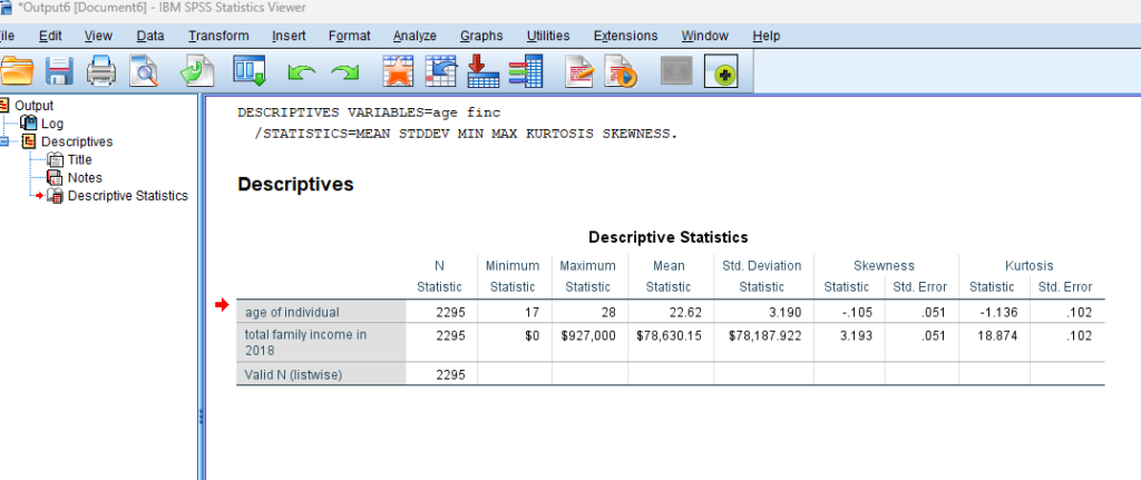
How to Interpret SPSS Output of Descriptive Statistics

Interpreting the SPSS output for descriptive statistics is pivotal for drawing meaningful conclusions. Firstly, focus on the measures of central tendency , such as the mean, median, and mode. These values provide insights into the typical or average score in your dataset. Next, examine measures of variability, including the range and standard deviation. The range indicates the spread of scores from the lowest to the highest, while the standard deviation quantifies the average amount of variation in your data.

SPSS Statistics for Descriptive

In our example, SPSS Output for Descriptive Statistics, the descriptive statistics provided describe two variables: “age of individual” and “total family income in 2018” based on a sample of 2295 individuals. Here’s an interpretation of age statistic:

Age of Individual:

• Mean : The average age of the individuals in the sample is approximately 22.62 years.
• Standard Deviation : The standard deviation of the ages is 3.190, indicating the extent of variability or dispersion around the mean.
• Skewness : The skewness is approximately -0.105. A negative skewness suggests that the distribution of ages is slightly skewed to the left, meaning there may be a longer tail on the left side of the distribution.
• Kurtosis : The kurtosis is -1.136. A negative kurtosis indicates that the distribution has lighter tails and is slightly less peaked than a normal distribution.

These descriptive statistics provide a summary of the central tendency, variability, skewness, and kurtosis for both the ages in the dataset.

How to Report Results of Descriptive Statistics in APA

Accurate reporting of descriptive statistics is crucial, especially when adhering to the guidelines of the American Psychological Association (APA). When presenting results, start with a brief description of the sample, including the total number of participants and any relevant demographics. Subsequently, report the key descriptive statistics, such as means and standard deviations, in a concise and organised manner. Ensure clarity by using appropriate tables and figures, and be mindful of APA formatting rules for statistical notation. Importantly, supplement your numerical results with brief interpretations, highlighting significant findings and their implications. By following APA guidelines, your reporting becomes not just a presentation of numbers but a narrative that communicates the story embedded within your data.

Example of Descriptive Statistics Results in APA Style

Embark on a seamless research journey with SPSSAnalysis.com , where our dedicated team provides expert data analysis assistance for students, academicians, and individuals. We ensure your research is elevated with precision. Explore our pages;

• SPSS Data Analysis Help – SPSS Helper ,
• Quantitative Analysis Help ,
• Qualitative Analysis Help ,
• SPSS Dissertation Analysis Help ,
• Dissertation Statistics Help ,
• Statistical Analysis Help ,
• Medical Data Analysis Help .

Connect with us at SPSSAnalysis.com to empower your research endeavors and achieve impactful results. Get a Free Quote Today !

Expert SPSS data analysis assistance available.