case study business size statistics

• All Headlines

Top 40 Most Popular Case Studies of 2021

Two cases about Hertz claimed top spots in 2021's Top 40 Most Popular Case Studies

Two cases on the uses of debt and equity at Hertz claimed top spots in the CRDT’s (Case Research and Development Team) 2021 top 40 review of cases.

Hertz (A) took the top spot. The case details the financial structure of the rental car company through the end of 2019. Hertz (B), which ranked third in CRDT’s list, describes the company’s struggles during the early part of the COVID pandemic and its eventual need to enter Chapter 11 bankruptcy. 

The success of the Hertz cases was unprecedented for the top 40 list. Usually, cases take a number of years to gain popularity, but the Hertz cases claimed top spots in their first year of release. Hertz (A) also became the first ‘cooked’ case to top the annual review, as all of the other winners had been web-based ‘raw’ cases.

Besides introducing students to the complicated financing required to maintain an enormous fleet of cars, the Hertz cases also expanded the diversity of case protagonists. Kathyrn Marinello was the CEO of Hertz during this period and the CFO, Jamere Jackson is black.

Sandwiched between the two Hertz cases, Coffee 2016, a perennial best seller, finished second. “Glory, Glory, Man United!” a case about an English football team’s IPO made a surprise move to number four.  Cases on search fund boards, the future of malls,  Norway’s Sovereign Wealth fund, Prodigy Finance, the Mayo Clinic, and Cadbury rounded out the top ten.

Other year-end data for 2021 showed:

• Online “raw” case usage remained steady as compared to 2020 with over 35K users from 170 countries and all 50 U.S. states interacting with 196 cases.
• Fifty four percent of raw case users came from outside the U.S..
• The Yale School of Management (SOM) case study directory pages received over 160K page views from 177 countries with approximately a third originating in India followed by the U.S. and the Philippines.
• Twenty-six of the cases in the list are raw cases.
• A third of the cases feature a woman protagonist.
• Orders for Yale SOM case studies increased by almost 50% compared to 2020.
• The top 40 cases were supervised by 19 different Yale SOM faculty members, several supervising multiple cases.

CRDT compiled the Top 40 list by combining data from its case store, Google Analytics, and other measures of interest and adoption.

All of this year’s Top 40 cases are available for purchase from the Yale Management Media store .

And the Top 40 cases studies of 2021 are:

1.   Hertz Global Holdings (A): Uses of Debt and Equity

2.   Coffee 2016

3.   Hertz Global Holdings (B): Uses of Debt and Equity 2020

4.   Glory, Glory Man United!

5.   Search Fund Company Boards: How CEOs Can Build Boards to Help Them Thrive

6.   The Future of Malls: Was Decline Inevitable?

7.   Strategy for Norway's Pension Fund Global

8.   Prodigy Finance

9.   Design at Mayo

10. Cadbury

11. City Hospital Emergency Room

13. Volkswagen

14. Marina Bay Sands

15. Shake Shack IPO

16. Mastercard

17. Netflix

18. Ant Financial

19. AXA: Creating the New CR Metrics

20. IBM Corporate Service Corps

21. Business Leadership in South Africa's 1994 Reforms

22. Alternative Meat Industry

23. Children's Premier

24. Khalil Tawil and Umi (A)

25. Palm Oil 2016

26. Teach For All: Designing a Global Network

27. What's Next? Search Fund Entrepreneurs Reflect on Life After Exit

28. Searching for a Search Fund Structure: A Student Takes a Tour of Various Options

30. Project Sammaan

31. Commonfund ESG

32. Polaroid

33. Connecticut Green Bank 2018: After the Raid

34. FieldFresh Foods

35. The Alibaba Group

36. 360 State Street: Real Options

37. Herman Miller

38. AgBiome

39. Nathan Cummings Foundation

40. Toyota 2010

We will keep fighting for all libraries - stand with us!

Internet Archive Audio

• This Just In
• Grateful Dead
• Old Time Radio
• 78 RPMs and Cylinder Recordings
• Audio Books & Poetry
• Computers, Technology and Science
• Music, Arts & Culture
• News & Public Affairs
• Spirituality & Religion
• Radio News Archive

• Flickr Commons
• Occupy Wall Street Flickr
• NASA Images
• Solar System Collection
• Ames Research Center

• All Software
• Old School Emulation
• MS-DOS Games
• Historical Software
• Classic PC Games
• Software Library
• Kodi Archive and Support File
• Vintage Software
• CD-ROM Software
• CD-ROM Software Library
• Software Sites
• Tucows Software Library
• Shareware CD-ROMs
• Software Capsules Compilation
• CD-ROM Images
• ZX Spectrum
• DOOM Level CD

• Smithsonian Libraries
• FEDLINK (US)
• Lincoln Collection
• American Libraries
• Canadian Libraries
• Universal Library
• Project Gutenberg
• Children's Library
• Biodiversity Heritage Library
• Books by Language
• Additional Collections

• Prelinger Archives
• Democracy Now!
• Occupy Wall Street
• TV NSA Clip Library
• Animation & Cartoons
• Arts & Music
• Computers & Technology
• Cultural & Academic Films
• Ephemeral Films
• Sports Videos
• Videogame Videos
• Youth Media

Search the history of over 866 billion web pages on the Internet.

Mobile Apps

• Wayback Machine (iOS)
• Wayback Machine (Android)

Browser Extensions

Archive-it subscription.

• Explore the Collections
• Build Collections

Save Page Now

Capture a web page as it appears now for use as a trusted citation in the future.

Please enter a valid web address

• Donate Donate icon An illustration of a heart shape

Practical data analysis : case studies in business statistics

Bookreader item preview, share or embed this item, flag this item for.

• Graphic Violence
• Explicit Sexual Content
• Hate Speech
• Misinformation/Disinformation
• Marketing/Phishing/Advertising
• Misleading/Inaccurate/Missing Metadata

plus-circle Add Review comment Reviews

212 Previews

3 Favorites

DOWNLOAD OPTIONS

No suitable files to display here.

PDF access not available for this item.

IN COLLECTIONS

Uploaded by station16.cebu on October 22, 2020

SIMILAR ITEMS (based on metadata)

Introduction to Statistical Thinking

Chapter 16 case studies, 16.1 student learning objective.

This chapter concludes this book. We start with a short review of the topics that were discussed in the second part of the book, the part that dealt with statistical inference. The main part of the chapter involves the statistical analysis of 2 case studies. The tools that will be used for the analysis are those that were discussed in the book. We close this chapter and this book with some concluding remarks. By the end of this chapter, the student should be able to:

Review the concepts and methods for statistical inference that were presented in the second part of the book.

Apply these methods to requirements of the analysis of real data.

Develop a resolve to learn more statistics.

16.2 A Review

The second part of the book dealt with statistical inference; the science of making general statement on an entire population on the basis of data from a sample. The basis for the statements are theoretical models that produce the sampling distribution. Procedures for making the inference are evaluated based on their properties in the context of this sampling distribution. Procedures with desirable properties are applied to the data. One may attach to the output of this application summaries that describe these theoretical properties.

In particular, we dealt with two forms of making inference. One form was estimation and the other was hypothesis testing. The goal in estimation is to determine the value of a parameter in the population. Point estimates or confidence intervals may be used in order to fulfill this goal. The properties of point estimators may be assessed using the mean square error (MSE) and the properties of the confidence interval may be assessed using the confidence level.

The target in hypotheses testing is to decide between two competing hypothesis. These hypotheses are formulated in terms of population parameters. The decision rule is called a statistical test and is constructed with the aid of a test statistic and a rejection region. The default hypothesis among the two, is rejected if the test statistic falls in the rejection region. The major property a test must possess is a bound on the probability of a Type I error, the probability of erroneously rejecting the null hypothesis. This restriction is called the significance level of the test. A test may also be assessed in terms of it’s statistical power, the probability of rightfully rejecting the null hypothesis.

Estimation and testing were applied in the context of single measurements and for the investigation of the relations between a pair of measurements. For single measurements we considered both numeric variables and factors. For numeric variables one may attempt to conduct inference on the expectation and/or the variance. For factors we considered the estimation of the probability of obtaining a level, or, more generally, the probability of the occurrence of an event.

We introduced statistical models that may be used to describe the relations between variables. One of the variables was designated as the response. The other variable, the explanatory variable, is identified as a variable which may affect the distribution of the response. Specifically, we considered numeric variables and factors that have two levels. If the explanatory variable is a factor with two levels then the analysis reduces to the comparison of two sub-populations, each one associated with a level. If the explanatory variable is numeric then a regression model may be applied, either linear or logistic regression, depending on the type of the response.

The foundations of statistical inference are the assumption that we make in the form of statistical models. These models attempt to reflect reality. However, one is advised to apply healthy skepticism when using the models. First, one should be aware what the assumptions are. Then one should ask oneself how reasonable are these assumption in the context of the specific analysis. Finally, one should check as much as one can the validity of the assumptions in light of the information at hand. It is useful to plot the data and compare the plot to the assumptions of the model.

16.3 Case Studies

Let us apply the methods that were introduced throughout the book to two examples of data analysis. Both examples are taken from the case studies of the Rice Virtual Lab in Statistics can be found in their Case Studies section. The analysis of these case studies may involve any of the tools that were described in the second part of the book (and some from the first part). It may be useful to read again Chapters  9 – 15 before reading the case studies.

16.3.1 Physicians’ Reactions to the Size of a Patient

Overweight and obesity is common in many of the developed contrives. In some cultures, obese individuals face discrimination in employment, education, and relationship contexts. The current research, conducted by Mikki Hebl and Jingping Xu 87 , examines physicians’ attitude toward overweight and obese patients in comparison to their attitude toward patients who are not overweight.

The experiment included a total of 122 primary care physicians affiliated with one of three major hospitals in the Texas Medical Center of Houston. These physicians were sent a packet containing a medical chart similar to the one they view upon seeing a patient. This chart portrayed a patient who was displaying symptoms of a migraine headache but was otherwise healthy. Two variables (the gender and the weight of the patient) were manipulated across six different versions of the medical charts. The weight of the patient, described in terms of Body Mass Index (BMI), was average (BMI = 23), overweight (BMI = 30), or obese (BMI = 36). Physicians were randomly assigned to receive one of the six charts, and were asked to look over the chart carefully and complete two medical forms. The first form asked physicians which of 42 tests they would recommend giving to the patient. The second form asked physicians to indicate how much time they believed they would spend with the patient, and to describe the reactions that they would have toward this patient.

In this presentation, only the question on how much time the physicians believed they would spend with the patient is analyzed. Although three patient weight conditions were used in the study (average, overweight, and obese) only the average and overweight conditions will be analyzed. Therefore, there are two levels of patient weight (average and overweight) and one dependent variable (time spent).

The data for the given collection of responses from 72 primary care physicians is stored in the file “ discriminate.csv ” 88 . We start by reading the content of the file into a data frame by the name “ patient ” and presenting the summary of the variables:

Observe that of the 72 “patients”, 38 are overweight and 33 have an average weight. The time spend with the patient, as predicted by physicians, is distributed between 5 minutes and 1 hour, with a average of 27.82 minutes and a median of 30 minutes.

It is a good practice to have a look at the data before doing the analysis. In this examination on should see that the numbers make sense and one should identify special features of the data. Even in this very simple example we may want to have a look at the histogram of the variable “ time ”:

A feature in this plot that catches attention is the fact that there is a high concventration of values in the interval between 25 and 30. Together with the fact that the median is equal to 30, one may suspect that, as a matter of fact, a large numeber of the values are actually equal to 30. Indeed, let us produce a table of the response:

Notice that 30 of the 72 physicians marked “ 30 ” as the time they expect to spend with the patient. This is the middle value in the range, and may just be the default value one marks if one just needs to complete a form and do not really place much importance to the question that was asked.

The goal of the analysis is to examine the relation between overweigh and the Doctor’s response. The explanatory variable is a factor with two levels. The response is numeric. A natural tool to use in order to test this hypothesis is the \(t\) -test, which is implemented with the function “ t.test ”.

First we plot the relation between the response and the explanatory variable and then we apply the test:

Nothing seems problematic in the box plot. The two distributions, as they are reflected in the box plots, look fairly symmetric.

When we consider the report that produced by the function “ t.test ” we may observe that the \(p\) -value is equal to 0.005774. This \(p\) -value is computed in testing the null hypothesis that the expectation of the response for both types of patients are equal against the two sided alternative. Since the \(p\) -value is less than 0.05 we do reject the null hypothesis.

The estimated value of the difference between the expectation of the response for a patient with BMI=23 and a patient with BMI=30 is \(31.36364 -24.73684 \approx 6.63\) minutes. The confidence interval is (approximately) equal to \([1.99, 11.27]\) . Hence, it looks as if the physicians expect to spend more time with the average weight patients.

After analyzing the effect of the explanatory variable on the expectation of the response one may want to examine the presence, or lack thereof, of such effect on the variance of the response. Towards that end, one may use the function “ var.test ”:

In this test we do not reject the null hypothesis that the two variances of the response are equal since the \(p\) -value is larger than \(0.05\) . The sample variances are almost equal to each other (their ratio is \(1.044316\) ), with a confidence interval for the ration that essentially ranges between 1/2 and 2.

The production of \(p\) -values and confidence intervals is just one aspect in the analysis of data. Another aspect, which typically is much more time consuming and requires experience and healthy skepticism is the examination of the assumptions that are used in order to produce the \(p\) -values and the confidence intervals. A clear violation of the assumptions may warn the statistician that perhaps the computed nominal quantities do not represent the actual statistical properties of the tools that were applied.

In this case, we have noticed the high concentration of the response at the value “ 30 ”. What is the situation when we split the sample between the two levels of the explanatory variable? Let us apply the function “ table ” once more, this time with the explanatory variable included:

Not surprisingly, there is still high concentration at that level “ 30 ”. But one can see that only 2 of the responses of the “ BMI=30 ” group are above that value in comparison to a much more symmetric distribution of responses for the other group.

The simulations of the significance level of the one-sample \(t\) -test for an Exponential response that were conducted in Question  \[ex:Testing.2\] may cast some doubt on how trustworthy are nominal \(p\) -values of the \(t\) -test when the measurements are skewed. The skewness of the response for the group “ BMI=30 ” is a reason to be worry.

We may consider a different test, which is more robust, in order to validate the significance of our findings. For example, we may turn the response into a factor by setting a level for values larger or equal to “ 30 ” and a different level for values less than “ 30 ”. The relation between the new response and the explanatory variable can be examined with the function “ prop.test ”. We first plot and then test:

The mosaic plot presents the relation between the explanatory variable and the new factor. The level “ TRUE ” is associated with a value of the predicted time spent with the patient being 30 minutes or more. The level “ FALSE ” is associated with a prediction of less than 30 minutes.

The computed \(p\) -value is equal to \(0.05409\) , that almost reaches the significance level of 5% 89 . Notice that the probabilities that are being estimated by the function are the probabilities of the level “ FALSE ”. Overall, one may see the outcome of this test as supporting evidence for the conclusion of the \(t\) -test. However, the \(p\) -value provided by the \(t\) -test may over emphasize the evidence in the data for a significant difference in the physician attitude towards overweight patients.

16.3.2 Physical Strength and Job Performance

The next case study involves an attempt to develop a measure of physical ability that is easy and quick to administer, does not risk injury, and is related to how well a person performs the actual job. The current example is based on study by Blakely et al.  90 , published in the journal Personnel Psychology.

There are a number of very important jobs that require, in addition to cognitive skills, a significant amount of strength to be able to perform at a high level. Construction worker, electrician and auto mechanic, all require strength in order to carry out critical components of their job. An interesting applied problem is how to select the best candidates from amongst a group of applicants for physically demanding jobs in a safe and a cost effective way.

The data presented in this case study, and may be used for the development of a method for selection among candidates, were collected from 147 individuals working in physically demanding jobs. Two measures of strength were gathered from each participant. These included grip and arm strength. A piece of equipment known as the Jackson Evaluation System (JES) was used to collect the strength data. The JES can be configured to measure the strength of a number of muscle groups. In this study, grip strength and arm strength were measured. The outcomes of these measurements were summarized in two scores of physical strength called “ grip ” and “ arm ”.

Two separate measures of job performance are presented in this case study. First, the supervisors for each of the participants were asked to rate how well their employee(s) perform on the physical aspects of their jobs. This measure is summarizes in the variable “ ratings ”. Second, simulations of physically demanding work tasks were developed. The summary score of these simulations are given in the variable “ sims ”. Higher values of either measures of performance indicates better performance.

The data for the 4 variables and 147 observations is stored in “ job.csv ” 91 . We start by reading the content of the file into a data frame by the name “ job ”, presenting a summary of the variables, and their histograms:

All variables are numeric. Examination of the 4 summaries and histograms does not produce interest findings. All variables are, more or less, symmetric with the distribution of the variable “ ratings ” tending perhaps to be more uniform then the other three.

The main analyses of interest are attempts to relate the two measures of physical strength “ grip ” and “ arm ” with the two measures of job performance, “ ratings ” and “ sims ”. A natural tool to consider in this context is a linear regression analysis that relates a measure of physical strength as an explanatory variable to a measure of job performance as a response.

FIGURE 16.1: Scatter Plots and Regression Lines

Let us consider the variable “ sims ” as a response. The first step is to plot a scatter plot of the response and explanatory variable, for both explanatory variables. To the scatter plot we add the line of regression. In order to add the regression line we fit the regression model with the function “ lm ” and then apply the function “ abline ” to the fitted model. The plot for the relation between the response and the variable “ grip ” is produced by the code:

The plot that is produced by this code is presented on the upper-left panel of Figure  16.1 .

The plot for the relation between the response and the variable “ arm ” is produced by this code:

The plot that is produced by the last code is presented on the upper-right panel of Figure  16.1 .

Both plots show similar characteristics. There is an overall linear trend in the relation between the explanatory variable and the response. The value of the response increases with the increase in the value of the explanatory variable (a positive slope). The regression line seems to follow, more or less, the trend that is demonstrated by the scatter plot.

A more detailed analysis of the regression model is possible by the application of the function “ summary ” to the fitted model. First the case where the explanatory variable is “ grip ”:

Examination of the report reviles a clear statistical significance for the effect of the explanatory variable on the distribution of response. The value of R-squared, the ration of the variance of the response explained by the regression is \(0.4094\) . The square root of this quantity, \(\sqrt{0.4094} \approx 0.64\) , is the proportion of the standard deviation of the response that is explained by the explanatory variable. Hence, about 64% of the variability in the response can be attributed to the measure of the strength of the grip.

For the variable “ arm ” we get:

This variable is also statistically significant. The value of R-squared is \(0.4706\) . The proportion of the standard deviation that is explained by the strength of the are is \(\sqrt{0.4706} \approx 0.69\) , which is slightly higher than the proportion explained by the grip.

Overall, the explanatory variables do a fine job in the reduction of the variability of the response “ sims ” and may be used as substitutes of the response in order to select among candidates. A better prediction of the response based on the values of the explanatory variables can be obtained by combining the information in both variables. The production of such combination is not discussed in this book, though it is similar in principle to the methods of linear regression that are presented in Chapter  14 . The produced score 92 takes the form:

\[\mbox{\texttt{score}} = -5.434 + 0.024\cdot \mbox{\texttt{grip}}+ 0.037\cdot \mbox{\texttt{arm}}\;.\] We use this combined score as an explanatory variable. First we form the score and plot the relation between it and the response:

The scatter plot that includes the regression line can be found at the lower-left panel of Figure  16.1 . Indeed, the linear trend is more pronounced for this scatter plot and the regression line a better description of the relation between the response and the explanatory variable. A summary of the regression model produces the report:

Indeed, the score is highly significant. More important, the R-squared coefficient that is associated with the score is \(0.5422\) , which corresponds to a ratio of the standard deviation that is explained by the model of \(\sqrt{0.5422} \approx 0.74\) . Thus, almost 3/4 of the variability is accounted for by the score, so the score is a reasonable mean of guessing what the results of the simulations will be. This guess is based only on the results of the simple tests of strength that is conducted with the JES device.

Before putting the final seal on the results let us examine the assumptions of the statistical model. First, with respect to the two explanatory variables. Does each of them really measure a different property or do they actually measure the same phenomena? In order to examine this question let us look at the scatter plot that describes the relation between the two explanatory variables. This plot is produced using the code:

It is presented in the lower-right panel of Figure  16.1 . Indeed, one may see that the two measurements of strength are not independent of each other but tend to produce an increasing linear trend. Hence, it should not be surprising that the relation of each of them with the response produces essentially the same goodness of fit. The computed score gives a slightly improved fit, but still, it basically reflects either of the original explanatory variables.

In light of this observation, one may want to consider other measures of strength that represents features of the strength not captures by these two variable. Namely, measures that show less joint trend than the two considered.

Another element that should be examined are the probabilistic assumptions that underly the regression model. We described the regression model only in terms of the functional relation between the explanatory variable and the expectation of the response. In the case of linear regression, for example, this relation was given in terms of a linear equation. However, another part of the model corresponds to the distribution of the measurements about the line of regression. The assumption that led to the computation of the reported \(p\) -values is that this distribution is Normal.

A method that can be used in order to investigate the validity of the Normal assumption is to analyze the residuals from the regression line. Recall that these residuals are computed as the difference between the observed value of the response and its estimated expectation, namely the fitted regression line. The residuals can be computed via the application of the function “ residuals ” to the fitted regression model.

Specifically, let us look at the residuals from the regression line that uses the score that is combined from the grip and arm measurements of strength. One may plot a histogram of the residuals:

The produced histogram is represented on the upper panel. The histogram portrays a symmetric distribution that my result from Normally distributed observations. A better method to compare the distribution of the residuals to the Normal distribution is to use the Quantile-Quantile plot . This plot can be found on the lower panel. We do not discuss here the method by which this plot is produced 93 . However, we do say that any deviation of the points from a straight line is indication of violation of the assumption of Normality. In the current case, the points seem to be on a single line, which is consistent with the assumptions of the regression model.

The next task should be an analysis of the relations between the explanatory variables and the other response “ ratings ”. In principle one may use the same steps that were presented for the investigation of the relations between the explanatory variables and the response “ sims ”. But of course, the conclusion may differ. We leave this part of the investigation as an exercise to the students.

16.4 Summary

16.4.1 concluding remarks.

The book included a description of some elements of statistics, element that we thought are simple enough to be explained as part of an introductory course to statistics and are the minimum that is required for any person that is involved in academic activities of any field in which the analysis of data is required. Now, as you finish the book, it is as good time as any to say some words regarding the elements of statistics that are missing from this book.

One element is more of the same. The statistical models that were presented are as simple as a model can get. A typical application will required more complex models. Each of these models may require specific methods for estimation and testing. The characteristics of inference, e.g. significance or confidence levels, rely on assumptions that the models are assumed to possess. The user should be familiar with computational tools that can be used for the analysis of these more complex models. Familiarity with the probabilistic assumptions is required in order to be able to interpret the computer output, to diagnose possible divergence from the assumptions and to assess the severity of the possible effect of such divergence on the validity of the findings.

Statistical tools can be used for tasks other than estimation and hypothesis testing. For example, one may use statistics for prediction. In many applications it is important to assess what the values of future observations may be and in what range of values are they likely to occur. Statistical tools such as regression are natural in this context. However, the required task is not testing or estimation the values of parameters, but the prediction of future values of the response.

A different role of statistics in the design stage. We hinted in that direction when we talked about in Chapter  \[ch:Confidence\] about the selection of a sample size in order to assure a confidence interval with a given accuracy. In most applications, the selection of the sample size emerges in the context of hypothesis testing and the criteria for selection is the minimal power of the test, a minimal probability to detect a true finding. Yet, statistical design is much more than the determination of the sample size. Statistics may have a crucial input in the decision of how to collect the data. With an eye on the requirements for the final analysis, an experienced statistician can make sure that data that is collected is indeed appropriate for that final analysis. Too often is the case where researcher steps into the statistician’s office with data that he or she collected and asks, when it is already too late, for help in the analysis of data that cannot provide a satisfactory answer to the research question the researcher tried to address. It may be said, with some exaggeration, that good statisticians are required for the final analysis only in the case where the initial planning was poor.

Last, but not least, is the theoretical mathematical theory of statistics. We tried to introduce as little as possible of the relevant mathematics in this course. However, if one seriously intends to learn and understand statistics then one must become familiar with the relevant mathematical theory. Clearly, deep knowledge in the mathematical theory of probability is required. But apart from that, there is a rich and rapidly growing body of research that deals with the mathematical aspects of data analysis. One cannot be a good statistician unless one becomes familiar with the important aspects of this theory.

I should have started the book with the famous quotation: “Lies, damned lies, and statistics”. Instead, I am using it to end the book. Statistics can be used and can be misused. Learning statistics can give you the tools to tell the difference between the two. My goal in writing the book is achieved if reading it will mark for you the beginning of the process of learning statistics and not the end of the process.

16.4.2 Discussion in the Forum

In the second part of the book we have learned many subjects. Most of these subjects, especially for those that had no previous exposure to statistics, were unfamiliar. In this forum we would like to ask you to share with us the difficulties that you encountered.

What was the topic that was most difficult for you to grasp? In your opinion, what was the source of the difficulty?

When forming your answer to this question we will appreciate if you could elaborate and give details of what the problem was. Pointing to deficiencies in the learning material and confusing explanations will help us improve the presentation for the future editions of this book.

Hebl, M. and Xu, J. (2001). Weighing the care: Physicians’ reactions to the size of a patient. International Journal of Obesity, 25, 1246-1252. ↩

The file can be found on the internet at http://pluto.huji.ac.il/~msby/StatThink/Datasets/discriminate.csv . ↩

One may propose splinting the response into two groups, with one group being associated with values of “ time ” strictly larger than 30 minutes and the other with values less or equal to 30. The resulting \(p\) -value from the expression “ prop.test(table(patient$time>30,patient$weight)) ” is \(0.01276\) . However, the number of subjects in one of the cells of the table is equal only to 2, which is problematic in the context of the Normal approximation that is used by this test. ↩

Blakley, B.A., Qui?ones, M.A., Crawford, M.S., and Jago, I.A. (1994). The validity of isometric strength tests. Personnel Psychology, 47, 247-274. ↩

The file can be found on the internet at http://pluto.huji.ac.il/~msby/StatThink/Datasets/job.csv . ↩

The score is produced by the application of the function “ lm ” to both variables as explanatory variables. The code expression that can be used is “ lm(sims ~ grip + arm, data=job) ”. ↩

Generally speaking, the plot is composed of the empirical percentiles of the residuals, plotted against the theoretical percentiles of the standard Normal distribution. The current plot is produced by the expression “ qqnorm(residuals(sims.score)) ”. ↩

How to write a case study — examples, templates, and tools

It’s a marketer’s job to communicate the effectiveness of a product or service to potential and current customers to convince them to buy and keep business moving. One of the best methods for doing this is to share success stories that are relatable to prospects and customers based on their pain points, experiences, and overall needs.

That’s where case studies come in. Case studies are an essential part of a content marketing plan. These in-depth stories of customer experiences are some of the most effective at demonstrating the value of a product or service. Yet many marketers don’t use them, whether because of their regimented formats or the process of customer involvement and approval.

A case study is a powerful tool for showcasing your hard work and the success your customer achieved. But writing a great case study can be difficult if you’ve never done it before or if it’s been a while. This guide will show you how to write an effective case study and provide real-world examples and templates that will keep readers engaged and support your business.

In this article, you’ll learn:

What is a case study?

How to write a case study, case study templates, case study examples, case study tools.

A case study is the detailed story of a customer’s experience with a product or service that demonstrates their success and often includes measurable outcomes. Case studies are used in a range of fields and for various reasons, from business to academic research. They’re especially impactful in marketing as brands work to convince and convert consumers with relatable, real-world stories of actual customer experiences.

The best case studies tell the story of a customer’s success, including the steps they took, the results they achieved, and the support they received from a brand along the way. To write a great case study, you need to:

• Celebrate the customer and make them — not a product or service — the star of the story.
• Craft the story with specific audiences or target segments in mind so that the story of one customer will be viewed as relatable and actionable for another customer.
• Write copy that is easy to read and engaging so that readers will gain the insights and messages intended.
• Follow a standardized format that includes all of the essentials a potential customer would find interesting and useful.
• Support all of the claims for success made in the story with data in the forms of hard numbers and customer statements.

Case studies are a type of review but more in depth, aiming to show — rather than just tell — the positive experiences that customers have with a brand. Notably, 89% of consumers read reviews before deciding to buy, and 79% view case study content as part of their purchasing process. When it comes to B2B sales, 52% of buyers rank case studies as an important part of their evaluation process.

Telling a brand story through the experience of a tried-and-true customer matters. The story is relatable to potential new customers as they imagine themselves in the shoes of the company or individual featured in the case study. Showcasing previous customers can help new ones see themselves engaging with your brand in the ways that are most meaningful to them.

Besides sharing the perspective of another customer, case studies stand out from other content marketing forms because they are based on evidence. Whether pulling from client testimonials or data-driven results, case studies tend to have more impact on new business because the story contains information that is both objective (data) and subjective (customer experience) — and the brand doesn’t sound too self-promotional.

Case studies are unique in that there’s a fairly standardized format for telling a customer’s story. But that doesn’t mean there isn’t room for creativity. It’s all about making sure that teams are clear on the goals for the case study — along with strategies for supporting content and channels — and understanding how the story fits within the framework of the company’s overall marketing goals.

Here are the basic steps to writing a good case study.

1. Identify your goal

Start by defining exactly who your case study will be designed to help. Case studies are about specific instances where a company works with a customer to achieve a goal. Identify which customers are likely to have these goals, as well as other needs the story should cover to appeal to them.

The answer is often found in one of the buyer personas that have been constructed as part of your larger marketing strategy. This can include anything from new leads generated by the marketing team to long-term customers that are being pressed for cross-sell opportunities. In all of these cases, demonstrating value through a relatable customer success story can be part of the solution to conversion.

2. Choose your client or subject

Who you highlight matters. Case studies tie brands together that might otherwise not cross paths. A writer will want to ensure that the highlighted customer aligns with their own company’s brand identity and offerings. Look for a customer with positive name recognition who has had great success with a product or service and is willing to be an advocate.

The client should also match up with the identified target audience. Whichever company or individual is selected should be a reflection of other potential customers who can see themselves in similar circumstances, having the same problems and possible solutions.

Some of the most compelling case studies feature customers who:

• Switch from one product or service to another while naming competitors that missed the mark.
• Experience measurable results that are relatable to others in a specific industry.
• Represent well-known brands and recognizable names that are likely to compel action.
• Advocate for a product or service as a champion and are well-versed in its advantages.

Whoever or whatever customer is selected, marketers must ensure they have the permission of the company involved before getting started. Some brands have strict review and approval procedures for any official marketing or promotional materials that include their name. Acquiring those approvals in advance will prevent any miscommunication or wasted effort if there is an issue with their legal or compliance teams.

3. Conduct research and compile data

Substantiating the claims made in a case study — either by the marketing team or customers themselves — adds validity to the story. To do this, include data and feedback from the client that defines what success looks like. This can be anything from demonstrating return on investment (ROI) to a specific metric the customer was striving to improve. Case studies should prove how an outcome was achieved and show tangible results that indicate to the customer that your solution is the right one.

This step could also include customer interviews. Make sure that the people being interviewed are key stakeholders in the purchase decision or deployment and use of the product or service that is being highlighted. Content writers should work off a set list of questions prepared in advance. It can be helpful to share these with the interviewees beforehand so they have time to consider and craft their responses. One of the best interview tactics to keep in mind is to ask questions where yes and no are not natural answers. This way, your subject will provide more open-ended responses that produce more meaningful content.

4. Choose the right format

There are a number of different ways to format a case study. Depending on what you hope to achieve, one style will be better than another. However, there are some common elements to include, such as:

• An engaging headline
• A subject and customer introduction
• The unique challenge or challenges the customer faced
• The solution the customer used to solve the problem
• The results achieved
• Data and statistics to back up claims of success
• A strong call to action (CTA) to engage with the vendor

It’s also important to note that while case studies are traditionally written as stories, they don’t have to be in a written format. Some companies choose to get more creative with their case studies and produce multimedia content, depending on their audience and objectives. Case study formats can include traditional print stories, interactive web or social content, data-heavy infographics, professionally shot videos, podcasts, and more.

5. Write your case study

We’ll go into more detail later about how exactly to write a case study, including templates and examples. Generally speaking, though, there are a few things to keep in mind when writing your case study.

• Be clear and concise. Readers want to get to the point of the story quickly and easily, and they’ll be looking to see themselves reflected in the story right from the start.
• Provide a big picture. Always make sure to explain who the client is, their goals, and how they achieved success in a short introduction to engage the reader.
• Construct a clear narrative. Stick to the story from the perspective of the customer and what they needed to solve instead of just listing product features or benefits.
• Leverage graphics. Incorporating infographics, charts, and sidebars can be a more engaging and eye-catching way to share key statistics and data in readable ways.
• Offer the right amount of detail. Most case studies are one or two pages with clear sections that a reader can skim to find the information most important to them.
• Include data to support claims. Show real results — both facts and figures and customer quotes — to demonstrate credibility and prove the solution works.

6. Promote your story

Marketers have a number of options for distribution of a freshly minted case study. Many brands choose to publish case studies on their website and post them on social media. This can help support SEO and organic content strategies while also boosting company credibility and trust as visitors see that other businesses have used the product or service.

Marketers are always looking for quality content they can use for lead generation. Consider offering a case study as gated content behind a form on a landing page or as an offer in an email message. One great way to do this is to summarize the content and tease the full story available for download after the user takes an action.

Sales teams can also leverage case studies, so be sure they are aware that the assets exist once they’re published. Especially when it comes to larger B2B sales, companies often ask for examples of similar customer challenges that have been solved.

Now that you’ve learned a bit about case studies and what they should include, you may be wondering how to start creating great customer story content. Here are a couple of templates you can use to structure your case study.

Template 1 — Challenge-solution-result format

• Start with an engaging title. This should be fewer than 70 characters long for SEO best practices. One of the best ways to approach the title is to include the customer’s name and a hint at the challenge they overcame in the end.
• Create an introduction. Lead with an explanation as to who the customer is, the need they had, and the opportunity they found with a specific product or solution. Writers can also suggest the success the customer experienced with the solution they chose.
• Present the challenge. This should be several paragraphs long and explain the problem the customer faced and the issues they were trying to solve. Details should tie into the company’s products and services naturally. This section needs to be the most relatable to the reader so they can picture themselves in a similar situation.
• Share the solution. Explain which product or service offered was the ideal fit for the customer and why. Feel free to delve into their experience setting up, purchasing, and onboarding the solution.
• Explain the results. Demonstrate the impact of the solution they chose by backing up their positive experience with data. Fill in with customer quotes and tangible, measurable results that show the effect of their choice.
• Ask for action. Include a CTA at the end of the case study that invites readers to reach out for more information, try a demo, or learn more — to nurture them further in the marketing pipeline. What you ask of the reader should tie directly into the goals that were established for the case study in the first place.

Template 2 — Data-driven format

• Start with an engaging title. Be sure to include a statistic or data point in the first 70 characters. Again, it’s best to include the customer’s name as part of the title.
• Create an overview. Share the customer’s background and a short version of the challenge they faced. Present the reason a particular product or service was chosen, and feel free to include quotes from the customer about their selection process.
• Present data point 1. Isolate the first metric that the customer used to define success and explain how the product or solution helped to achieve this goal. Provide data points and quotes to substantiate the claim that success was achieved.
• Present data point 2. Isolate the second metric that the customer used to define success and explain what the product or solution did to achieve this goal. Provide data points and quotes to substantiate the claim that success was achieved.
• Present data point 3. Isolate the final metric that the customer used to define success and explain what the product or solution did to achieve this goal. Provide data points and quotes to substantiate the claim that success was achieved.
• Summarize the results. Reiterate the fact that the customer was able to achieve success thanks to a specific product or service. Include quotes and statements that reflect customer satisfaction and suggest they plan to continue using the solution.
• Ask for action. Include a CTA at the end of the case study that asks readers to reach out for more information, try a demo, or learn more — to further nurture them in the marketing pipeline. Again, remember that this is where marketers can look to convert their content into action with the customer.

While templates are helpful, seeing a case study in action can also be a great way to learn. Here are some examples of how Adobe customers have experienced success.

Juniper Networks

One example is the Adobe and Juniper Networks case study , which puts the reader in the customer’s shoes. The beginning of the story quickly orients the reader so that they know exactly who the article is about and what they were trying to achieve. Solutions are outlined in a way that shows Adobe Experience Manager is the best choice and a natural fit for the customer. Along the way, quotes from the client are incorporated to help add validity to the statements. The results in the case study are conveyed with clear evidence of scale and volume using tangible data.

The story of Lenovo’s journey with Adobe is one that spans years of planning, implementation, and rollout. The Lenovo case study does a great job of consolidating all of this into a relatable journey that other enterprise organizations can see themselves taking, despite the project size. This case study also features descriptive headers and compelling visual elements that engage the reader and strengthen the content.

Tata Consulting

When it comes to using data to show customer results, this case study does an excellent job of conveying details and numbers in an easy-to-digest manner. Bullet points at the start break up the content while also helping the reader understand exactly what the case study will be about. Tata Consulting used Adobe to deliver elevated, engaging content experiences for a large telecommunications client of its own — an objective that’s relatable for a lot of companies.

Case studies are a vital tool for any marketing team as they enable you to demonstrate the value of your company’s products and services to others. They help marketers do their job and add credibility to a brand trying to promote its solutions by using the experiences and stories of real customers.

When you’re ready to get started with a case study:

• Think about a few goals you’d like to accomplish with your content.
• Make a list of successful clients that would be strong candidates for a case study.
• Reach out to the client to get their approval and conduct an interview.
• Gather the data to present an engaging and effective customer story.

Adobe can help

There are several Adobe products that can help you craft compelling case studies. Adobe Experience Platform helps you collect data and deliver great customer experiences across every channel. Once you’ve created your case studies, Experience Platform will help you deliver the right information to the right customer at the right time for maximum impact.

To learn more, watch the Adobe Experience Platform story .

Keep in mind that the best case studies are backed by data. That’s where Adobe Real-Time Customer Data Platform and Adobe Analytics come into play. With Real-Time CDP, you can gather the data you need to build a great case study and target specific customers to deliver the content to the right audience at the perfect moment.

Watch the Real-Time CDP overview video to learn more.

Finally, Adobe Analytics turns real-time data into real-time insights. It helps your business collect and synthesize data from multiple platforms to make more informed decisions and create the best case study possible.

Request a demo to learn more about Adobe Analytics.

https://business.adobe.com/blog/perspectives/b2b-ecommerce-10-case-studies-inspire-you

https://business.adobe.com/blog/basics/business-case

https://business.adobe.com/blog/basics/what-is-real-time-analytics

• SUGGESTED TOPICS
• The Magazine
• Newsletters
• Managing Yourself
• Managing Teams
• Work-life Balance
• The Big Idea
• Data & Visuals
• Reading Lists
• Case Selections
• HBR Learning
• Topic Feeds
• Account Settings
• Email Preferences

HBS Case Selections

OpenAI: Idealism Meets Capitalism

• Shikhar Ghosh
• Shweta Bagai

Generative AI and the Future of Work

• Christopher Stanton
• Matt Higgins

Copilot(s): Generative AI at Microsoft and GitHub

• Frank Nagle
• Shane Greenstein
• Maria P. Roche
• Nataliya Langburd Wright
• Sarah Mehta

Innovation at Moog Inc.

• Brian J. Hall
• Ashley V. Whillans
• Davis Heniford
• Dominika Randle
• Caroline Witten

Innovation at Google Ads: The Sales Acceleration and Innovation Labs (SAIL) (A)

• Linda A. Hill
• Emily Tedards

Juan Valdez: Innovation in Caffeination

• Michael I. Norton
• Jeremy Dann

UGG Steps into the Metaverse

• Shunyuan Zhang
• Sharon Joseph
• Sunil Gupta
• Julia Kelley

Metaverse Wars

• David B. Yoffie

Roblox: Virtual Commerce in the Metaverse

• Ayelet Israeli
• Nicole Tempest Keller

Timnit Gebru: "SILENCED No More" on AI Bias and The Harms of Large Language Models

• Tsedal Neeley
• Stefani Ruper

Hugging Face: Serving AI on a Platform

• Kerry Herman
• Sarah Gulick

SmartOne: Building an AI Data Business

• Karim R. Lakhani
• Pippa Tubman Armerding
• Gamze Yucaoglu
• Fares Khrais

Honeywell and the Great Recession (A)

• Sandra J. Sucher
• Susan Winterberg

Target: Responding to the Recession

• Ranjay Gulati
• Catherine Ross
• Richard S. Ruback
• Royce Yudkoff

Hometown Foods: Changing Price Amid Inflation

• Julian De Freitas
• Jeremy Yang
• Das Narayandas

Elon Musk's Big Bets

• Eric Baldwin

Elon Musk: Balancing Purpose and Risk

Tesla's ceo compensation plan.

• Krishna G. Palepu
• John R. Wells
• Gabriel Ellsworth

China Rapid Finance: The Collapse of China's P2P Lending Industry

• William C. Kirby
• Bonnie Yining Cao
• John P. McHugh

Forbidden City: Launching a Craft Beer in China

• Christopher A. Bartlett
• Carole Carlson

Booking.com

• Stefan Thomke
• Daniela Beyersdorfer

Innovation at Uber: The Launch of Express POOL

• Chiara Farronato
• Alan MacCormack

Racial Discrimination on Airbnb (A)

• Michael Luca
• Scott Stern
• Hyunjin Kim

Unilever's Response to the Future of Work

• William R. Kerr
• Emilie Billaud
• Mette Fuglsang Hjortshoej

AT&T, Retraining, and the Workforce of Tomorrow

• Joseph B. Fuller
• Carl Kreitzberg

Leading Change in Talent at L'Oreal

• Lakshmi Ramarajan
• Vincent Dessain
• Emer Moloney
• William W. George
• Andrew N. McLean

Eve Hall: The African American Investment Fund in Milwaukee

• Steven S. Rogers
• Alterrell Mills

United Housing - Otis Gates

• Mercer Cook

The Home Depot: Leadership in Crisis Management

• Herman B. Leonard
• Marc J. Epstein
• Melissa Tritter

The Great East Japan Earthquake (B): Fast Retailing Group's Response

• Hirotaka Takeuchi
• Kenichi Nonomura
• Dena Neuenschwander
• Meghan Ricci
• Kate Schoch
• Sergey Vartanov

Insurer of Last Resort?: The Federal Financial Response to September 11

• David A. Moss
• Sarah Brennan

Under Armour

• Rory McDonald
• Clayton M. Christensen
• Daniel West
• Jonathan E. Palmer
• Tonia Junker

Hunley, Inc.: Casting for Growth

• John A. Quelch
• James T. Kindley

Bitfury: Blockchain for Government

• Mitchell B. Weiss
• Elena Corsi

Deutsche Bank: Pursuing Blockchain Opportunities (A)

• Lynda M. Applegate
• Christoph Muller-Bloch

Maersk: Betting on Blockchain

• Scott Johnson

Yum! Brands

• Jordan Siegel
• Christopher Poliquin

Bharti Airtel in Africa

• Tanya Bijlani

Li & Fung 2012

• F. Warren McFarlan
• Michael Shih-ta Chen
• Keith Chi-ho Wong

Sony and the JK Wedding Dance

• John Deighton
• Leora Kornfeld

United Breaks Guitars

David dao on united airlines.

• Benjamin Edelman
• Jenny Sanford

Marketing Reading: Digital Marketing

• Joseph Davin

Social Strategy at Nike

• Mikolaj Jan Piskorski
• Ryan Johnson

The Tate's Digital Transformation

Social strategy at american express, mellon financial and the bank of new york.

• Carliss Y. Baldwin
• Ryan D. Taliaferro

The Walt Disney Company and Pixar, Inc.: To Acquire or Not to Acquire?

• Juan Alcacer
• David J. Collis

Dow's Bid for Rohm and Haas

• Benjamin C. Esty

Finance Reading: The Mergers and Acquisitions Process

• John Coates

Apple: Privacy vs. Safety? (A)

• Henry W. McGee
• Nien-he Hsieh
• Sarah McAra

Sidewalk Labs: Privacy in a City Built from the Internet Up

• Leslie K. John

Data Breach at Equifax

• Suraj Srinivasan
• Quinn Pitcher
• Jonah S. Goldberg

Apple's Core

• Noam Wasserman

Design Thinking and Innovation at Apple

• Barbara Feinberg

Apple Inc. in 2012

• Penelope Rossano

Iz-Lynn Chan at Far East Organization (Abridged)

• Anthony J. Mayo
• Dana M. Teppert

Barbara Norris: Leading Change in the General Surgery Unit

• Boris Groysberg
• Nitin Nohria
• Deborah Bell

Adobe Systems: Working Towards a "Suite" Release (A)

• David A. Thomas
• Lauren Barley

Home Nursing of North Carolina

Castronics, llc, gemini investors, angie's list: ratings pioneer turns 20.

• Robert J. Dolan

Basecamp: Pricing

• Frank V. Cespedes
• Robb Fitzsimmons

J.C. Penney's "Fair and Square" Pricing Strategy

J.c. penney's 'fair and square' strategy (c): back to the future.

• Jose B. Alvarez

Osaro: Picking the best path

• James Palano
• Bastiane Huang

HubSpot and Motion AI: Chatbot-Enabled CRM

• Thomas Steenburgh

GROW: Using Artificial Intelligence to Screen Human Intelligence

• Ethan S. Bernstein
• Paul D. McKinnon
• Paul Yarabe

Arup: Building the Water Cube

• Robert G. Eccles
• Amy C. Edmondson
• Dilyana Karadzhova

(Re)Building a Global Team: Tariq Khan at Tek

Managing a global team: greg james at sun microsystems, inc. (a).

• Thomas J. DeLong

Organizational Behavior Reading: Leading Global Teams

Ron ventura at mitchell memorial hospital.

• Heide Abelli

Anthony Starks at InSiL Therapeutics (A)

• Gary P. Pisano
• Vicki L. Sato

Wolfgang Keller at Konigsbrau-TAK (A)

• John J. Gabarro

Midland Energy Resources, Inc.: Cost of Capital

• Timothy A. Luehrman
• Joel L. Heilprin

Globalizing the Cost of Capital and Capital Budgeting at AES

• Mihir A. Desai
• Doug Schillinger

Cost of Capital at Ameritrade

• Mark Mitchell
• Erik Stafford

Finance Reading: Cost of Capital

David Neeleman: Flight Path of a Servant Leader (A)

• Matthew D. Breitfelder

Coach Hurley at St. Anthony High School

• Scott A. Snook
• Bradley C. Lawrence

Shapiro Global

• Michael Brookshire
• Monica Haugen
• Michelle Kravetz
• Sarah Sommer

Kathryn McNeil (A)

• Joseph L. Badaracco Jr.
• Jerry Useem

Carol Fishman Cohen: Professional Career Reentry (A)

• Myra M. Hart
• Robin J. Ely
• Susan Wojewoda

Alex Montana at ESH Manufacturing Co.

• Michael Kernish

Michelle Levene (A)

• Tiziana Casciaro
• Victoria W. Winston

John and Andrea Rice: Entrepreneurship and Life

• Howard H. Stevenson
• Janet Kraus
• Shirley M. Spence

Partner Center

• Research Guides
• Case Studies and Statistics
• Company and Industry Resources
• Business News
• Business OER

Case Studies in Marketing

• Encyclopedia of Major Marketing Campaigns Profiles important marketing campaigns.
• Cases in Advertising Management Covers advertising management in 34 companies.
• Cases in Sport Marketing Covers 14 marketing campaigns in sports and sporting goods.
• Marketing Management: Text and Cases A textbook with many case examples.
• Experiential Marketing : Case Studies in Customer Experience An ebook with 36 case studies in customer experience.
• Valuable Content Marketing : How to Make Quality Content Your Key to Success Valuable Content Marketing shows how to create and share valuable content on websites and through social media and more traditional methods.

Business Statistics: Library Databases

Business statistics: web sites.

• ClickZ Internet Stats and Demographics Statistics on Internet use and trends.
• Surveys of Consumers
• Pew Research Center
• << Previous: Company and Industry Resources
• Next: Business News >>
• Last Updated: May 8, 2024 9:16 AM
• URL: https://library.uhd.edu/business

7 Favorite Business Case Studies to Teach—and Why

Explore more.

• Case Teaching
• Course Materials

FEATURED CASE STUDIES

The Army Crew Team . Emily Michelle David of CEIBS

ATH Technologies . Devin Shanthikumar of Paul Merage School of Business

Fabritek 1992 . Rob Austin of Ivey Business School

Lincoln Electric Co . Karin Schnarr of Wilfrid Laurier University

Pal’s Sudden Service—Scaling an Organizational Model to Drive Growth . Gary Pisano of Harvard Business School

The United States Air Force: ‘Chaos’ in the 99th Reconnaissance Squadron . Francesca Gino of Harvard Business School

Warren E. Buffett, 2015 . Robert F. Bruner of Darden School of Business

To dig into what makes a compelling case study, we asked seven experienced educators who teach with—and many who write—business case studies: “What is your favorite case to teach and why?”

The resulting list of case study favorites ranges in topics from operations management and organizational structure to rebel leaders and whodunnit dramas.

1. The Army Crew Team

Emily Michelle David, Assistant Professor of Management, China Europe International Business School (CEIBS)

“I love teaching  The Army Crew Team  case because it beautifully demonstrates how a team can be so much less than the sum of its parts.

I deliver the case to executives in a nearby state-of-the-art rowing facility that features rowing machines, professional coaches, and shiny red eight-person shells.

After going through the case, they hear testimonies from former members of Chinese national crew teams before carrying their own boat to the river for a test race.

The rich learning environment helps to vividly underscore one of the case’s core messages: competition can be a double-edged sword if not properly managed.

Executives in Emily Michelle David’s organizational behavior class participate in rowing activities at a nearby facility as part of her case delivery.

Despite working for an elite headhunting firm, the executives in my most recent class were surprised to realize how much they’ve allowed their own team-building responsibilities to lapse. In the MBA pre-course, this case often leads to a rich discussion about common traps that newcomers fall into (for example, trying to do too much, too soon), which helps to poise them to both stand out in the MBA as well as prepare them for the lateral team building they will soon engage in.

Finally, I love that the post-script always gets a good laugh and serves as an early lesson that organizational behavior courses will seldom give you foolproof solutions for specific problems but will, instead, arm you with the ability to think through issues more critically.”

2. ATH Technologies

Devin Shanthikumar, Associate Professor of Accounting, Paul Merage School of Business

“As a professor at UC Irvine’s Paul Merage School of Business, and before that at Harvard Business School, I have probably taught over 100 cases. I would like to say that my favorite case is my own,   Compass Box Whisky Company . But as fun as that case is, one case beats it:  ATH Technologies  by Robert Simons and Jennifer Packard.

ATH presents a young entrepreneurial company that is bought by a much larger company. As part of the merger, ATH gets an ‘earn-out’ deal—common among high-tech industries. The company, and the class, must decide what to do to achieve the stretch earn-out goals.

ATH captures a scenario we all want to be in at some point in our careers—being part of a young, exciting, growing organization. And a scenario we all will likely face—having stretch goals that seem almost unreachable.

It forces us, as a class, to really struggle with what to do at each stage.

After we read and discuss the A case, we find out what happens next, and discuss the B case, then the C, then D, and even E. At every stage, we can:

see how our decisions play out,

figure out how to build on our successes, and

address our failures.

The case is exciting, the class discussion is dynamic and energetic, and in the end, we all go home with a memorable ‘ah-ha!’ moment.

I have taught many great cases over my career, but none are quite as fun, memorable, and effective as ATH .”

3. Fabritek 1992

Rob Austin, Professor of Information Systems, Ivey Business School

“This might seem like an odd choice, but my favorite case to teach is an old operations case called  Fabritek 1992 .

The latest version of Fabritek 1992 is dated 2009, but it is my understanding that this is a rewrite of a case that is older (probably much older). There is a Fabritek 1969 in the HBP catalog—same basic case, older dates, and numbers. That 1969 version lists no authors, so I suspect the case goes even further back; the 1969 version is, I’m guessing, a rewrite of an even older version.

There are many things I appreciate about the case. Here are a few:

It operates as a learning opportunity at many levels. At first it looks like a not-very-glamorous production job scheduling case. By the end of the case discussion, though, we’re into (operations) strategy and more. It starts out technical, then explodes into much broader relevance. As I tell participants when I’m teaching HBP's Teaching with Cases seminars —where I often use Fabritek as an example—when people first encounter this case, they almost always underestimate it.

It has great characters—especially Arthur Moreno, who looks like a troublemaker, but who, discussion reveals, might just be the smartest guy in the factory. Alums of the Harvard MBA program have told me that they remember Arthur Moreno many years later.

Almost every word in the case is important. It’s only four and a half pages of text and three pages of exhibits. This economy of words and sparsity of style have always seemed like poetry to me. I should note that this super concise, every-word-matters approach is not the ideal we usually aspire to when we write cases. Often, we include extra or superfluous information because part of our teaching objective is to provide practice in separating what matters from what doesn’t in a case. Fabritek takes a different approach, though, which fits it well.

It has a dramatic structure. It unfolds like a detective story, a sort of whodunnit. Something is wrong. There is a quality problem, and we’re not sure who or what is responsible. One person, Arthur Moreno, looks very guilty (probably too obviously guilty), but as we dig into the situation, there are many more possibilities. We spend in-class time analyzing the data (there’s a bit of math, so it covers that base, too) to determine which hypotheses are best supported by the data. And, realistically, the data doesn’t support any of the hypotheses perfectly, just some of them more than others. Also, there’s a plot twist at the end (I won’t reveal it, but here’s a hint: Arthur Moreno isn’t nearly the biggest problem in the final analysis). I have had students tell me the surprising realization at the end of the discussion gives them ‘goosebumps.’

Finally, through the unexpected plot twist, it imparts what I call a ‘wisdom lesson’ to young managers: not to be too sure of themselves and to regard the experiences of others, especially experts out on the factory floor, with great seriousness.”

4. Lincoln Electric Co.

Karin Schnarr, Assistant Professor of Policy, Wilfrid Laurier University

“As a strategy professor, my favorite case to teach is the classic 1975 Harvard case  Lincoln Electric Co.  by Norman Berg.

I use it to demonstrate to students the theory linkage between strategy and organizational structure, management processes, and leadership behavior.

This case may be an odd choice for a favorite. It occurs decades before my students were born. It is pages longer than we are told students are now willing to read. It is about manufacturing arc welding equipment in Cleveland, Ohio—a hard sell for a Canadian business classroom.

Yet, I have never come across a case that so perfectly illustrates what I want students to learn about how a company can be designed from an organizational perspective to successfully implement its strategy.

And in a time where so much focus continues to be on how to maximize shareholder value, it is refreshing to be able to discuss a publicly-traded company that is successfully pursuing a strategy that provides a fair value to shareholders while distributing value to employees through a large bonus pool, as well as value to customers by continually lowering prices.

However, to make the case resonate with today’s students, I work to make it relevant to the contemporary business environment. I link the case to multimedia clips about Lincoln Electric’s current manufacturing practices, processes, and leadership practices. My students can then see that a model that has been in place for generations is still viable and highly successful, even in our very different competitive situation.”

5. Pal’s Sudden Service—Scaling an Organizational Model to Drive Growth

Gary Pisano, Professor of Business Administration, Harvard Business School

“My favorite case to teach these days is  Pal’s Sudden Service—Scaling an Organizational Model to Drive Growth .

I love teaching this case for three reasons:

1. It demonstrates how a company in a super-tough, highly competitive business can do very well by focusing on creating unique operating capabilities. In theory, Pal’s should have no chance against behemoths like McDonalds or Wendy’s—but it thrives because it has built a unique operating system. It’s a great example of a strategic approach to operations in action.

2. The case shows how a strategic approach to human resource and talent development at all levels really matters. This company competes in an industry not known for engaging its front-line workers. The case shows how engaging these workers can really pay off.

3. Finally, Pal’s is really unusual in its approach to growth. Most companies set growth goals (usually arbitrary ones) and then try to figure out how to ‘backfill’ the human resource and talent management gaps. They trust you can always find someone to do the job. Pal’s tackles the growth problem completely the other way around. They rigorously select and train their future managers. Only when they have a manager ready to take on their own store do they open a new one. They pace their growth off their capacity to develop talent. I find this really fascinating and so do the students I teach this case to.”

6. The United States Air Force: ‘Chaos’ in the 99th Reconnaissance Squadron

Francesca Gino, Professor of Business Administration, Harvard Business School

“My favorite case to teach is  The United States Air Force: ‘Chaos’ in the 99th Reconnaissance Squadron .

The case surprises students because it is about a leader, known in the unit by the nickname Chaos , who inspired his squadron to be innovative and to change in a culture that is all about not rocking the boat, and where there is a deep sense that rules should simply be followed.

For years, I studied ‘rebels,’ people who do not accept the status quo; rather, they approach work with curiosity and produce positive change in their organizations. Chaos is a rebel leader who got the level of cultural change right. Many of the leaders I’ve met over the years complain about the ‘corporate culture,’ or at least point to clear weaknesses of it; but then they throw their hands up in the air and forget about changing what they can.

Chaos is different—he didn’t go after the ‘Air Force’ culture. That would be like boiling the ocean.

Instead, he focused on his unit of control and command: The 99th squadron. He focused on enabling that group to do what it needed to do within the confines of the bigger Air Force culture. In the process, he inspired everyone on his team to be the best they can be at work.

The case leaves the classroom buzzing and inspired to take action.”

7. Warren E. Buffett, 2015

Robert F. Bruner, Professor of Business Administration, Darden School of Business

“I love teaching   Warren E. Buffett, 2015  because it energizes, exercises, and surprises students.

Buffett looms large in the business firmament and therefore attracts anyone who is eager to learn his secrets for successful investing. This generates the kind of energy that helps to break the ice among students and instructors early in a course and to lay the groundwork for good case discussion practices.

Studying Buffett’s approach to investing helps to introduce and exercise important themes that will resonate throughout a course. The case challenges students to define for themselves what it means to create value. The case discussion can easily be tailored for novices or for more advanced students.

Either way, this is not hero worship: The case affords a critical examination of the financial performance of Buffett’s firm, Berkshire Hathaway, and reveals both triumphs and stumbles. Most importantly, students can critique the purported benefits of Buffett’s conglomeration strategy and the sustainability of his investment record as the size of the firm grows very large.

By the end of the class session, students seem surprised with what they have discovered. They buzz over the paradoxes in Buffett’s philosophy and performance record. And they come away with sober respect for Buffett’s acumen and for the challenges of creating value for investors.

Surely, such sobriety is a meta-message for any mastery of finance.”

More Educator Favorites

Emily Michelle David is an assistant professor of management at China Europe International Business School (CEIBS). Her current research focuses on discovering how to make workplaces more welcoming for people of all backgrounds and personality profiles to maximize performance and avoid employee burnout. David’s work has been published in a number of scholarly journals, and she has worked as an in-house researcher at both NASA and the M.D. Anderson Cancer Center.

Devin Shanthikumar  is an associate professor and the accounting area coordinator at UCI Paul Merage School of Business. She teaches undergraduate, MBA, and executive-level courses in managerial accounting. Shanthikumar previously served on the faculty at Harvard Business School, where she taught both financial accounting and managerial accounting for MBAs, and wrote cases that are used in accounting courses across the country.

Robert D. Austin is a professor of information systems at Ivey Business School and an affiliated faculty member at Harvard Medical School. He has published widely, authoring nine books, more than 50 cases and notes, three Harvard online products, and two popular massive open online courses (MOOCs) running on the Coursera platform.

Karin Schnarr is an assistant professor of policy and the director of the Bachelor of Business Administration (BBA) program at the Lazaridis School of Business & Economics at Wilfrid Laurier University in Waterloo, Ontario, Canada where she teaches strategic management at the undergraduate, graduate, and executive levels. Schnarr has published several award-winning and best-selling cases and regularly presents at international conferences on case writing and scholarship.

Gary P. Pisano is the Harry E. Figgie, Jr. Professor of Business Administration and senior associate dean of faculty development at Harvard Business School, where he has been on the faculty since 1988. Pisano is an expert in the fields of technology and operations strategy, the management of innovation, and competitive strategy. His research and consulting experience span a range of industries including aerospace, biotechnology, pharmaceuticals, specialty chemicals, health care, nutrition, computers, software, telecommunications, and semiconductors.

Francesca Gino studies how people can have more productive, creative, and fulfilling lives. She is a professor at Harvard Business School and the author, most recently, of  Rebel Talent: Why It Pays to Break the Rules at Work and in Life . Gino regularly gives keynote speeches, delivers corporate training programs, and serves in advisory roles for firms and not-for-profit organizations across the globe.

Robert F. Bruner is a university professor at the University of Virginia, distinguished professor of business administration, and dean emeritus of the Darden School of Business. He has also held visiting appointments at Harvard and Columbia universities in the United States, at INSEAD in France, and at IESE in Spain. He is the author, co-author, or editor of more than 20 books on finance, management, and teaching. Currently, he teaches and writes in finance and management.

Related Articles

We use cookies to understand how you use our site and to improve your experience, including personalizing content. Learn More . By continuing to use our site, you accept our use of cookies and revised Privacy Policy .

LEARN STATISTICS EASILY

Learn Data Analysis Now!

5 Statistics Case Studies That Will Blow Your Mind

You will learn the transformative impact of statistical science in unfolding real-world narratives from global economics to public health victories.

Introduction

The untrained eye may see only cold, lifeless digits in the intricate dance of numbers and patterns that constitute data analysis and statistics. Yet, for those who know how to listen, these numbers whisper stories about our world, our behaviors, and the delicate interplay of systems and relationships that shape our reality. Artfully unfolded through meticulous statistical analysis, these narratives can reveal startling truths and unseen correlations that challenge our understanding and broaden our horizons. Here are five case studies demonstrating the profound power of statistics to decode reality’s vast and complex tapestry.

• 2008 Financial Crisis : Regression analysis showed Lehman Brothers’ collapse rippled globally, causing a credit crunch and recession.
• Eradication of Guinea Worm Disease : Geospatial and logistic regression helped reduce cases from 3.5 million to 54 by 2019.
• Amazon’s Personalized Marketing : Machine learning algorithms predict customer preferences, drive sales, and set industry benchmarks for personalized shopping.
• American Bald Eagle Recovery : Statistical models and the DDT ban led to the recovery of the species, once on the brink of extinction.
• Twitter and Political Polarization : MIT’s sentiment analysis of tweets revealed echo chambers, influencing political discourse and highlighting the need for algorithm transparency.

1. The Butterfly Effect in Global Markets: The 2008 Financial Crisis

The 2008 financial crisis is a prime real-world example of the Butterfly Effect in global markets. What started as a crisis in the housing market in the United States quickly escalated into a full-blown international banking crisis with the collapse of the investment bank Lehman Brothers on September 15, 2008.

Understanding the Ripples

A team of economists employed regression analysis to understand the impact of the Lehman Brothers collapse. The statistical models revealed how this event affected financial institutions worldwide, causing a credit crunch and a widespread economic downturn.

The Data Weaves a Story

Further analysis using time-series forecasting methods painted a detailed picture of the crisis’s spread. For instance, these models were used to predict how the initial shockwave would impact housing markets globally, consumer spending, and unemployment rates. These forecasts proved incredibly accurate, showcasing not only the domino effect of the crisis but also the predictive power of well-crafted statistical models.

Implications for Future Predictions

This real-life event became a case study of the importance of understanding the deep connections within the global financial system. Banks, policymakers, and investors now use the predictive models developed from the 2008 crisis to stress-test economic systems against similar shocks. It has led to a greater appreciation of risk management and the implementation of stricter financial regulations to safeguard against future crises.

By interpreting the unfolding of the 2008 crisis through the lens of statistical science, we can appreciate the profound effect that one event in a highly interconnected system can have. The lessons learned continue to resonate, influencing financial policies and the global economic forecasting and stability approach.

2. Statistical Fortitude in Public Health: The Eradication of Dracunculiasis (Guinea Worm Disease)

In a world teeming with infectious diseases, the story of dracunculiasis, commonly known as Guinea Worm Disease, is a testament to public health tenacity and the judicious application of statistical analysis in disease eradication efforts.

Tracing the Path of the Parasite

The campaign against dracunculiasis, led by The Carter Center and supported by a consortium of international partners, utilized epidemiological data to trace and interrupt the life cycle of the Guinea worm — the statistical approach underpinning this public health victory involved meticulously collecting data on disease incidence and transmission patterns.

The Tally of Triumph

By employing geospatial statistics and logistic regression models, health workers pinpointed endemic villages and formulated strategies that targeted the disease’s transmission vectors. These statistical tools were instrumental in monitoring the progress of eradication efforts and allocating resources to areas most in need.

The Countdown to Zero

The eradication campaign’s success was measured by the continuous decline in cases, from an estimated 3.5 million in the mid-1980s to just 54 reported cases in 2019. This dramatic decrease has been documented through rigorous data collection and statistical validation, ensuring that each reported case was accounted for and dealt with accordingly.

Legacy of a Worm

The nearing eradication of Guinea Worm Disease, with no vaccine or curative treatment, is a feat that underscores the power of preventive public health strategies informed by statistical analysis. It serves as a blueprint for tackling other infectious diseases. It is a real-world example of how statistics can aid in making the invisible enemy of disease a known and conquerable foe.

The narrative of Guinea Worm eradication is not just a tale of statistical victory but also one of human resilience and commitment to public health. It is a story that will continue to inspire as the world edges closer to declaring dracunculiasis the second human disease, after smallpox, to be eradicated.

3. Unraveling the DNA of Consumer Behavior: A Case Study of Amazon’s Personalized Marketing

The advent of big data analytics has revolutionized marketing strategies by providing deep insights into consumer behavior. Amazon, a global leader in e-commerce, is at the forefront of leveraging statistical analysis to offer its customers a highly personalized shopping experience.

The Predictive Power of Purchase Patterns

Amazon collects vast user data, including browsing histories, purchase patterns, and product searches. Amazon analyzes this data by employing machine learning algorithms to predict individual customer preferences and future buying behavior. This predictive power is exemplified by Amazon’s recommendation engine, which suggests products to users with uncanny accuracy, often leading to increased sales and customer satisfaction.

Beyond the Purchase: Sentiment Analysis

Amazon extends its data analysis beyond purchases by analyzing customer reviews and feedback sentiment. This analysis gives Amazon a nuanced understanding of customer sentiments towards products and services. Amazon can quickly address issues, improve product offerings, and enhance customer service by mining text for customer sentiment.

Crafting Tomorrow’s Trends Today

Amazon’s data analytics insights are not limited to personalizing the shopping experience. They are also used to anticipate and set future trends. Amazon has mastered the art of using consumer data to meet existing demands and influence and create new consumer needs. By analyzing emerging patterns, Amazon stocks products ahead of demand spikes and develops new products that align with predicted consumer trends.

Amazon’s success in utilizing statistical analysis for marketing is a testament to the power of big data in shaping the future of consumer engagement. The company’s ability to personalize the shopping experience and anticipate consumer trends has set a benchmark in the industry, illustrating the transformative impact of statistics on marketing strategies.

4. The Revival of the American Bald Eagle: A Triumph of Environmental Policy and Statistics

In the annals of environmental success stories, the recovery of the American Bald Eagle (Haliaeetus leucocephalus) from extinction stands out as a sterling example of how rigorous science, public policy, and statistics can combine to safeguard wildlife. This case study offers a narrative that encapsulates the meticulous application of data analysis in wildlife conservation, revealing a more profound truth about the interdependence of species and the human spirit’s capacity for stewardship.

The Descent Towards Silence

By the mid-20th century, the American Bald Eagle, a symbol of freedom and strength, faced decimation. Pesticides like DDT, habitat loss, and illegal shooting had dramatically reduced their numbers. The alarming descent prompted an urgent call to action bolstered by the rigorous collection and analysis of ecological data.

The Statistical Lifeline

Biostatisticians and ecologists began a comprehensive monitoring program, recording eagle population numbers, nesting sites, and chick survival rates. Advanced statistical models, including logistic regression and population viability analysis (PVA), were employed to assess the eagles’ extinction risk under various scenarios and to evaluate the effectiveness of different conservation strategies.

The Ban on DDT – A Calculated Decision

A pivotal moment in the Bald Eagle’s story was the ban on DDT in 1972, a decision grounded in the statistical analysis of the pesticide’s impacts on eagle reproduction. Studies demonstrated a strong correlation between DDT and thinning eggshells, leading to reduced hatching rates. Based on this analysis, the ban’s implementation marked the turning point for the eagle’s fate.

A Soaring Recovery

Post-ban, rigorous monitoring continued, and the data collected painted a story of resilience and recovery. The statistical evidence was undeniable: eagle populations were rebounding. As of the early 21st century, the Bald Eagle had made a miraculous comeback, removed from the Endangered Species List in 2007.

The Legacy of a Species

The American Bald Eagle’s resurgence is more than a conservation narrative; it’s a testament to the harmony between humanity’s analytical prowess and its capacity for environmental guardianship. It shows how statistics can forecast doom and herald a new dawn for conservation. This case study epitomizes the beautiful interplay between human action, informed by truth and statistical insight, resulting in a tangible good: the return of a majestic species from the shadow of extinction.

5. The Algorithmic Mirrors of Social Media – The Case of Twitter and Political Polarization

Social media platforms, particularly Twitter, have become critical arenas for public discourse, shaping societal norms and reflecting public sentiment. This case study examines the real-world application of statistical models and algorithms to understand Twitter’s role in political polarization.

Twitter’s Data-Driven Sentiment Reflection

The aim was to analyze Twitter data to evaluate public sentiment regarding political events and understand the platform’s contribution to societal polarization.

Using natural language processing (NLP) and sentiment analysis, researchers from the Massachusetts Institute of Technology (MIT) analyzed over 10 million tweets from the period surrounding the 2020 U.S. Presidential Election. The tweets were filtered using politically relevant hashtags and keywords.

Deciphering the Digital Pulse

A sentiment index was created, categorizing tweets into positive, negative, or neutral sentiments concerning the candidates. This ‘Twitter Political Sentiment Index’ provided a temporal view of public mood swings about key campaign events and debates.

The Echo Chambers of the Internet

Network analysis revealed distinct user clusters along ideological lines, illustrating the presence of echo chambers. The study examined retweet networks and highlighted how information circulated within politically homogeneous groups, reinforcing existing beliefs.

The study showed limited user exposure to opposing political views on Twitter, increasing polarization. It also correlated significant shifts in the sentiment index with real-life events, such as policy announcements and election results.

Shaping the Future of Public Discourse

The study, published in Science, emphasizes the need for transparency in social media algorithms to mitigate echo chambers’ effects. The insights gained are being used to inform policymakers and educators about the dynamics of online discourse and to encourage the design of algorithms that promote a more balanced and open digital exchange of ideas.

The findings from MIT’s Twitter data analysis underscore the platform’s power as a real-time barometer of public sentiment and its role in shaping political discourse. The case study offers a roadmap for leveraging big data to foster a healthier democratic process in the digital age.

Drawing together these varied case studies, it becomes clear that statistics and data analysis are far from mere computation tools. They are, in fact, the instruments through which we can uncover deeper truths about our world. They can illuminate the unseen, predict the future, and help us shape it towards the common good. These narratives exemplify the pursuit of true knowledge, promoting good actions, and appreciating a beautiful world.

As we engage with the data of our daily lives, we continually decode the complexities of existence. From the markets to the microorganisms, consumer behavior to conservation efforts, and the physical to the digital world, statistics is the language in which the tales of our times are written. It is the language that reveals the integrity of systems, the harmony of nature, and the pulse of humanity. Through this science’s meticulous and ethical application, we uphold the values of truth, goodness, and beauty — ideals that remain ever-present in the quest for understanding and improving the world we share.

Recommended Articles

Curious about the untold stories behind the numbers? Dive into our blog for more riveting articles that showcase the transformative power of statistics in understanding and shaping our world. Continue your journey into the beauty of data-driven truths with us.

• Music, Tea, and P-Values: Impossible Results and P-Hacking
• Statistical Fallacies and the Perception of the Mozart Effect
• How Data Visualization in the Form of Pie Charts Saved Lives

Frequently Asked Questions

Q1: What is the significance of the 2008 Financial Crisis in statistics?  The 2008 Financial Crisis is significant in statistics for demonstrating the Butterfly Effect in global markets, where regression analysis revealed the interconnected impact of Lehman Brothers’ collapse on the global economy.

Q2: How did statistics contribute to the eradication of Guinea Worm Disease?  Through geospatial and logistic regression, statistics played a crucial role in tracking and reducing the spread of Guinea Worm Disease, contributing to the decline from 3.5 million cases to just 54 by 2019.

Q3: What role does machine learning play in Amazon’s marketing?  Machine learning algorithms at Amazon analyze vast amounts of consumer data to predict customer preferences and personalize the shopping experience, driving sales and setting industry benchmarks.

Q4: How were statistics instrumental in the recovery of the American Bald Eagle?  Statistical models helped assess the risk of extinction and the impact of DDT on eagle reproduction, leading to conservation strategies that aided in the eagle’s significant recovery.

Q5: What is sentiment analysis, and how was it used in studying Twitter?  Sentiment analysis uses natural language processing to categorize the tone of text content. MIT used it to evaluate political sentiment on Twitter and study the platform’s role in political polarization.

Q6: How did statistical models predict the global effects of the 2008 crisis?  Statistical models, including time-series forecasting, predicted how the crisis would affect housing markets, consumer spending, and unemployment, demonstrating the predictive power of statistics.

Q7: Why is the eradication of Guinea Worm Disease significant beyond public health?  The near eradication, without a vaccine or cure, illustrates the power of preventive strategies and statistical analysis in public health, serving as a blueprint for combating other diseases.

Q8: In what way did statistics aid in the decision to ban DDT?  Statistical analysis linked DDT to thinning eagle eggshells and poor hatching rates, leading to the ban crucial for the Bald Eagle’s recovery.

Q9: How does Amazon’s use of data analytics influence consumer behavior?  By analyzing consumer data, Amazon anticipates and sets trends, meets demands, and influences new consumer needs, shaping the future of consumer engagement.

Q10: What implications does the Twitter political polarization study have?  The study calls for transparency in social media algorithms to reduce echo chambers. It suggests using statistical insights to foster a balanced, open digital exchange in democratic processes.

Similar Posts

A Comprehensive Guide on Using a Percentage Table Calculator

Explore the world of percentage table calculators: their functions, applications, and best practices for accurate data analysis.

Applied Statistics: Data Analysis

If you’re struggling with statistics while analyzing data for your projects, this is your ultimate solution for Data Analysis!

Confounding Variables in Statistics: Strategies for Identifying and Adjusting

Explore how confounding variables in statistics can impact your research and learn effective strategies for identifying and adjusting them.

Design of Experiments: Elevating Research with Precision

Explore how ‘Design of Experiments’ optimizes research precision, enhancing truth and beauty in data analysis.

Outlier Detection and Treatment: A Comprehensive Guide

Master Outlier Detection and Treatment to enhance your data analysis skills. A definitive guide for data scientists seeking accuracy.

Statistics is the Grammar of Science

Discover why ‘Statistics is the grammar of Science’ and its pivotal role in driving scientific insights and breakthroughs.

Leave a Reply Cancel reply

Your email address will not be published. Required fields are marked *

Save my name, email, and website in this browser for the next time I comment.

Cookie Policy

We use cookies to operate this website, improve usability, personalize your experience, and improve our marketing. Privacy Policy .

By clicking "Accept" or further use of this website, you agree to allow cookies.

• Data Science
• Data Analytics
• Machine Learning

Essential Statistics for Data Science: A Case Study using Python, Part I

Get to know some of the essential statistics you should be very familiar with when learning data science

LearnDataSci is reader-supported. When you purchase through links on our site, earned commissions help support our team of writers, researchers, and designers at no extra cost to you.

Our last post dove straight into linear regression. In this post, we'll take a step back to cover essential statistics that every data scientist should know. To demonstrate these essentials, we'll look at a hypothetical case study involving an administrator tasked with improving school performance in Tennessee.

You should already know:

• Python fundamentals — learn on dataquest.io

Note, this tutorial is intended to serve solely as an educational tool and not as a scientific explanation of the causes of various school outcomes in Tennessee .

Article Resources

• Notebook and Data: Github
• Libraries: pandas, matplotlib, seaborn

Introduction

Meet Sally, a public school administrator. Some schools in her state of Tennessee are performing below average academically. Her superintendent, under pressure from frustrated parents and voters, approached Sally with the task of understanding why these schools are under-performing. Not an easy problem, to be sure.

To improve school performance, Sally needs to learn more about these schools and their students, just as a business needs to understand its own strengths and weaknesses and its customers.

Though Sally is eager to build an impressive explanatory model, she knows the importance of conducting preliminary research to prevent possible pitfalls or blind spots (e.g. cognitive bias'). Thus, she engages in a thorough exploratory analysis, which includes: a lit review, data collection, descriptive and inferential statistics, and data visualization.

Sally has strong opinions as to why some schools are under-performing, but opinions won't do, nor will a handful of facts; she needs rigorous statistical evidence.

Sally conducts a lit review, which involves reading a variety of credible sources to familiarize herself with the topic. Most importantly, Sally keeps an open mind and embraces a scientific world view to help her resist confirmation bias (seeking solely to confirm one's own world view).

In Sally's lit review, she finds multiple compelling explanations of school performance: curriculae , income , and parental involvement . These sources will help Sally select her model and data, and will guide her interpretation of the results.

Data Collection

The data we want isn't always available, but Sally lucks out and finds student performance data based on test scores ( school_rating ) for every public school in middle Tennessee. The data also includes various demographic, school faculty, and income variables (see readme for more information). Satisfied with this dataset, she writes a web-scraper to retrieve the data.

But data alone can't help Sally; she needs to convert the data into useful information.

Descriptive and Inferential Statistics

Sally opens her stats textbook and finds that there are two major types of statistics, descriptive and inferential.

Descriptive statistics identify patterns in the data, but they don't allow for making hypotheses about the data.

Within descriptive statistics, there are two measures used to describe the data: central tendency and deviation . Central tendency refers to the central position of the data (mean, median, mode) while the deviation describes how far spread out the data are from the mean. Deviation is most commonly measured with the standard deviation. A small standard deviation indicates the data are close to the mean, while a large standard deviation indicates that the data are more spread out from the mean.

Inferential statistics allow us to make hypotheses (or inferences ) about a sample that can be applied to the population. For Sally, this involves developing a hypothesis about her sample of middle Tennessee schools and applying it to her population of all schools in Tennessee.

For now, Sally puts aside inferential statistics and digs into descriptive statistics.

To begin learning about the sample, Sally uses pandas' describe method, as seen below. The column headers in bold text represent the variables Sally will be exploring. Each row header represents a descriptive statistic about the corresponding column.

Looking at the output above, Sally's variables can be put into two classes: measurements and indicators.

Measurements are variables that can be quantified. All data in the output above are measurements. Some of these measurements, such as state_percentile_16 , avg_score_16 and school_rating , are outcomes; these outcomes cannot be used to explain one another. For example, explaining school_rating as a result of state_percentile_16 (test scores) is circular logic. Therefore we need a second class of variables.

The second class, indicators, are used to explain our outcomes. Sally chooses indicators that describe the student body (for example, reduced_lunch ) or school administration ( stu_teach_ratio ) hoping they will explain school_rating .

Sally sees a pattern in one of the indicators, reduced_lunch . reduced_lunch is a variable measuring the average percentage of students per school enrolled in a federal program that provides lunches for students from lower-income households. In short, reduced_lunch is a good proxy for household income, which Sally remembers from her lit review was correlated with school performance.

Sally isolates reduced_lunch and groups the data by school_rating using pandas' groupby method and then uses describe on the re-shaped data (see below).

Below is a discussion of the metrics from the table above and what each result indicates about the relationship between school_rating and reduced_lunch :

count : the number of schools at each rating. Most of the schools in Sally's sample have a 4- or 5-star rating, but 25% of schools have a 1-star rating or below. This confirms that poor school performance isn't merely anecdotal, but a serious problem that deserves attention.

mean : the average percentage of students on reduced_lunch among all schools by each school_rating . As school performance increases, the average number of students on reduced lunch decreases. Schools with a 0-star rating have 83.6% of students on reduced lunch. And on the other end of the spectrum, 5-star schools on average have 21.6% of students on reduced lunch. We'll examine this pattern further. in the graphing section.

std : the standard deviation of the variable. Referring to the school_rating of 0, a standard deviation of 8.813498 indicates that 68.2% (refer to readme ) of all observations are within 8.81 percentage points on either side of the average, 83.6%. Note that the standard deviation increases as school_rating increases, indicating that reduced_lunch loses explanatory power as school performance improves. As with the mean, we'll explore this idea further in the graphing section.

min : the minimum value of the variable. This represents the school with the lowest percentage of students on reduced lunch at each school rating. For 0- and 1-star schools, the minimum percentage of students on reduced lunch is 53%. The minimum for 5-star schools is 2%. The minimum value tells a similar story as the mean, but looking at it from the low end of the range of observations.

25% : the bottom quartile; represents the lowest 25% of values for the variable, reduced_lunch . For 0-star schools, 25% of the observations are less than 79.5%. Sally sees the same trend in the bottom quartile as the above metrics: as school_rating increases the bottom 25% of reduced_lunch decreases.

50% : the second quartile; represents the lowest 50% of values. Looking at the trend in school_rating and reduced_lunch , the same relationship is present here.

75% : the top quartile; represents the lowest 75% of values. The trend continues.

max : the maximum value for that variable. You guessed it: the trend continues!

The descriptive statistics consistently reveal that schools with more students on reduced lunch under-perform when compared to their peers. Sally is on to something.

Sally decides to look at reduced_lunch from another angle using a correlation matrix with pandas' corr method. The values in the correlation matrix table will be between -1 and 1 (see below). A value of -1 indicates the strongest possible negative correlation, meaning as one variable decreases the other increases. And a value of 1 indicates the opposite. The result below, -0.815757, indicates strong negative correlation between reduced_lunch and school_rating . There's clearly a relationship between the two variables.

Sally continues to explore this relationship graphically.

Essential Graphs for Exploring Data

Box-and-whisker plot.

In her stats book, Sally sees a box-and-whisker plot . A box-and-whisker plot is helpful for visualizing the distribution of the data from the mean. Understanding the distribution allows Sally to understand how far spread out her data is from the mean; the larger the spread from the mean, the less robust reduced_lunch is at explaining school_rating .

See below for an explanation of the box-and-whisker plot.

Now that Sally knows how to read the box-and-whisker plot, she graphs reduced_lunch to see the distributions. See below.

In her box-and-whisker plots, Sally sees that the minimum and maximum reduced_lunch values tend to get closer to the mean as school_rating decreases; that is, as school_rating decreases so does the standard deviation in reduced_lunch .

What does this mean?

Starting with the top box-and-whisker plot, as school_rating decreases, reduced_lunch becomes a more powerful way to explain outcomes. This could be because as parents' incomes decrease they have fewer resources to devote to their children's education (such as, after-school programs, tutors, time spent on homework, computer camps, etc) than higher-income parents. Above a 3-star rating, more predictors are needed to explain school_rating due to an increasing spread in reduced_lunch .

Having used box-and-whisker plots to reaffirm her idea that household income and school performance are related, Sally seeks further validation.

Scatter Plot

To further examine the relationship between school_rating and reduced_lunch , Sally graphs the two variables on a scatter plot. See below.

In the scatter plot above, each dot represents a school. The placement of the dot represents that school's rating (Y-axis) and the percentage of its students on reduced lunch (x-axis).

The downward trend line shows the negative correlation between school_rating and reduced_lunch (as one increases, the other decreases). The slope of the trend line indicates how much school_rating decreases as reduced_lunch increases. A steeper slope would indicate that a small change in reduced_lunch has a big impact on school_rating while a more horizontal slope would indicate that the same small change in reduced_lunch has a smaller impact on school_rating .

Sally notices that the scatter plot further supports what she saw with the box-and-whisker plot: when reduced_lunch increases, school_rating decreases. The tighter spread of the data as school_rating declines indicates the increasing influence of reduced_lunch . Now she has a hypothesis.

Correlation Matrix

Sally is ready to test her hypothesis: a negative relationship exists between school_rating and reduced_lunch (to be covered in a follow up article). If the test is successful, she'll need to build a more robust model using additional variables. If the test fails, she'll need to re-visit her dataset to choose other variables that possibly explain school_rating . Either way, Sally could benefit from an efficient way of assessing relationships among her variables.

An efficient graph for assessing relationships is the correlation matrix, as seen below; its color-coded cells make it easier to interpret than the tabular correlation matrix above. Red cells indicate positive correlation; blue cells indicate negative correlation; white cells indicate no correlation. The darker the colors, the stronger the correlation (positive or negative) between those two variables.

With the correlation matrix in mind as a future starting point for finding additional variables, Sally moves on for now and prepares to test her hypothesis.

Sally was approached with a problem: why are some schools in middle Tennessee under-performing? To answer this question, she did the following:

• Conducted a lit review to educate herself on the topic.
• Gathered data from a reputable source to explore school ratings and characteristics of the student bodies and schools in middle Tennessee.
• The data indicated a robust relationship between school_rating and reduced_lunch .
• Explored the data visually.
• Though satisfied with her preliminary findings, Sally is keeping her mind open to other explanations.
• Developed a hypothesis: a negative relationship exists between school_rating and reduced_lunch .

In a follow up article, Sally will test her hypothesis. Should she find a satisfactory explanation for her sample of schools, she will attempt to apply her explanation to the population of schools in Tennessee.

Course Recommendations

Further learning:, applied data science with python — coursera, statistics and data science micromasters — edx, get updates in your inbox.

Join over 7,500 data science learners.

Recent articles:

The 9 best ai courses for 2024 (and two to avoid), the 6 best python courses for 2024 – ranked by software engineer, best course deals for black friday and cyber monday 2024, sigmoid function, 7 best artificial intelligence (ai) courses.

Top courses you can take today to begin your journey into the Artificial Intelligence field.

Meet the Authors

A graduate of Belmont University, Tim is a Nashville, TN-based software engineer and statistician at Perception Health, an industry leader in healthcare analytics, and co-founder of Sidekick, LLC, a data consulting company. Find him on  Twitter  and  GitHub .

John is a research analyst at Laffer Associates, a macroeconomic consulting firm based in Nashville, TN. He graduated from Belmont University. Find him on  GitHub  and  LinkedIn

Back to blog index

A case study comparing machine learning with statistical methods for time series forecasting: size matters

• Published: 16 May 2022
• Volume 59 , pages 415–433, ( 2022 )

Cite this article

• Vitor Cerqueira 1 ,
• Luis Torgo 1 &
• Carlos Soares 2 , 3 , 4  

1171 Accesses

10 Citations

Explore all metrics

Time series forecasting is one of the most active research topics. Machine learning methods have been increasingly adopted to solve these predictive tasks. However, in a recent work, evidence was shown that these approaches systematically present a lower predictive performance relative to simple statistical methods. In this work, we counter these results. We show that these are only valid under an extremely low sample size. Using a learning curve method, our results suggest that machine learning methods improve their relative predictive performance as the sample size grows. The R code to reproduce all of our experiments is available at https://github.com/vcerqueira/MLforForecasting .

This is a preview of subscription content, log in via an institution to check access.

Access this article

Price includes VAT (Russian Federation)

Instant access to the full article PDF.

Rent this article via DeepDyve

Institutional subscriptions

Similar content being viewed by others

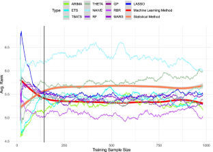
Machine Learning Strategies for Time Series Forecasting

Evaluating time series forecasting models: an empirical study on performance estimation methods

predtoolsTS: R package for streamlining time series forecasting

Data availability.

All experiments and data are publicly available (c.f. abstract)

Ahmed, N. K., Atiya, A. F., Gayar, N. E., & El-Shishiny, H. (2010). An empirical comparison of machine learning models for time series forecasting. Econometric Reviews , 29 (5-6), 594–621.

Article   MathSciNet   Google Scholar  

Assimakopoulos, V., & Nikolopoulos, K. (2000). The theta model: a decomposition approach to forecasting. International Journal of Forecasting, 16 (4), 521–530.

Article   Google Scholar  

Box, G. E., Jenkins, G. M., Reinsel, G. C., & Ljung, G. M. (2015). Time series analysis: forecasting and control . New York: John Wiley & Sons.

MATH   Google Scholar  

Breiman, L. (2001). Random forests. Machine Learning , 45 (1), 5–32.

Carbonneau, R., Laframboise, K., & Vahidov, R. (2008). Application of machine learning techniques for supply chain demand forecasting. European Journal of Operational Research , 184 (3), 1140–1154.

Cerqueira, V., Torgo, L., Pinto, F., & Soares, C. (2019). Arbitrage of forecasting experts. Machine Learning , 108 (6), 913–944.

Chatfield, C. (2000). Time-series forecasting. CRC Press.

Cleveland, W. S., Grosse, E., & Shyu, W. M. (2017). Local regression models. In Statistical models in s, pp. 309–376. Routledge .

Cox, D. R., & Stuart, A. (1955). Some quick sign tests for trend in location and dispersion. Biometrika , 42 (1/2), 80–95.

Dawid, A. P. (1984). Present position and potential developments: Some personal views statistical theory the prequential approach. Journal of the Royal Statistical Society: Series A (General) , 147 (2), 278–290.

De Livera, A. M., Hyndman, R. J., & Snyder, R. D. (2011). Forecasting time series with complex seasonal patterns using exponential smoothing. Journal of the American Statistical Association , 106 (496), 1513–1527.

Dietterich, T. G. (2002). Machine learning for sequential data: a review. In Joint IAPR international workshops on statistical techniques in pattern recognition (SPR) and structural and syntactic pattern recognition (SSPR), pp. 15–30. Springer .

Friedman, J., Hastie, T., & Tibshirani, R. (2010). Regularization paths for generalized linear models via coordinate descent. Journal of Statistical Software , 33 (1), 1–22.

Friedman, J. H., et al. (1991). Multivariate adaptive regression splines. The Annals of Statistics , 19 (1), 1–67.

MathSciNet   MATH   Google Scholar  

Gama, J. (2010). Knowledge discovery from data streams. Chapman and hall/CRC.

Gardner, E. S. Jr (1985). Exponential smoothing: The state of the art. Journal of Forecasting , 4 (1), 1–28.

Goodfellow, I., Bengio, Y., Courville, A., & Bengio, Y. (2016). Deep learning, vol. 1 MIT Press Cambridge.

Guerrero, V. M. (1993). Time-series analysis supported by power transformations. Journal of Forecasting , 12 (1), 37–48.

Hill, T., O’Connor, M., & Remus, W. (1996). Neural network models for time series forecasts. Management Science, 42 (7), 1082–1092.

Hyndman, R., & Yang, Y. (2019). tsdl: Time Series Data Library. https://finyang.github.io/tsdl/ .

Hyndman, R. J., & Athanasopoulos, G. (2018). Forecasting: principles and practice OTexts.

Hyndman, R.J. with contributions from George Athanasopoulos, Razbash, S., Schmidt, D., Zhou, Z., Khan, Y., Bergmeir, C., & Wang, E. (2014). forecast: Forecasting functions for time series and linear models. R package version 5.6.

Hyndman, R. J., & Koehler, A. B. (2006). Another look at measures of forecast accuracy. International Journal of Forecasting , 22 (4), 679–688.

Januschowski, T., Gasthaus, J., Wang, Y., Salinas, D., Flunkert, V., Bohlke-Schneider, M., & Callot, L. (2020). Criteria for classifying forecasting methods. International Journal of Forecasting , 36 (1), 167–177.

Karatzoglou, A., Smola, A., Hornik, K., & Zeileis, A. (2004). kernlab – an S4 package for kernel methods in R. Journal of Statistical Software , 11 (9), 1–20.

Kennel, M. B., Brown, R., & Abarbanel, H. D. (1992). Determining embedding dimension for phase-space reconstruction using a geometrical construction. Physical Review A , 45 (6), 3403.

Kilian, L., & Taylor, M. P. (2003). Why is it so difficult to beat the random walk forecast of exchange rates? Journal of International Economics , 60 (1), 85–107.

Kuhn, M., Weston, S., & Keefer, C. (2014). code for Cubist by Ross Quinlan, N.C.C.: Cubist: rule- and instance-based regression modeling. R package version 0.0.18.

Lee, J., & Mark, R. G. (2010). An investigation of patterns in hemodynamic data indicative of impending hypotension in intensive care. Biomedical Engineering Online , 9 (1), 62.

Makridakis, S., & Hibon, M. (1997). Arma models and the box–jenkins methodology. Journal of Forecasting , 16 (3), 147–163.

Makridakis, S., & Hibon, M. (2000). The m3-competition: results, conclusions and implications. International Journal of Forecasting , 16 (4), 451–476.

Makridakis, S., Spiliotis, E., & Assimakopoulos, V. (2018). Statistical and machine learning forecasting methods: Concerns and ways forward. PloS One , 13 (3), e0194,889.

McCullagh, P. (2019). Generalized linear models. Routledge.

Michalski, R., Carbonell, J., & Mitchell, T. (1983). Machine learning: An artificial intelligence approach.

Milborrow, S. (2016). earth: Multivariate adaptive regression splines. R package version 4.4.4.

Oreshkin, B. N., Carpov, D., Chapados, N., & Bengio, Y. (2019). N-beats: Neural basis expansion analysis for interpretable time series forecasting. arXiv: 1905.10437 .

Provost, F., Jensen, D., & Oates, T. (1999). Efficient progressive sampling. In Proceedings of the fifth ACM SIGKDD international conference on Knowledge discovery and data mining, pp. 23–32. ACM .

Quinlan, J. R. (1993). Combining instance-based and model-based learning. In Proceedings of the tenth international conference on machine learning, pp. 236–243 .

Spiliotis, E., Makridakis, S., Semenoglou, A. A., & Assimakopoulos, V. (2020). Comparison of statistical and machine learning methods for daily sku demand forecasting. Operational Research, 1–25.

Taieb, S. B., Bontempi, G., Atiya, A. F., & Sorjamaa, A. (2012). A review and comparison of strategies for multi-step ahead time series forecasting based on the nn5 forecasting competition. Expert Systems with Applications , 39 (8), 7067–7083.

Takens, F. (1981). Dynamical Systems and Turbulence. In Warwick 1980: Proceedings of a Symposium Held at the University of Warwick 1979/80, chap. Detecting strange attractors in turbulence (pp. 366–381). Berlin: Springer.

Taylor, S. J., & Letham, B. (2018). Forecasting at scale. The American Statistician , 72 (1), 37–45.

Voyant, C., Notton, G., Kalogirou, S., Nivet, M. L., Paoli, C., Motte, F., & Fouilloy, A. (2017). Machine learning methods for solar radiation forecasting: a review. Renewable Energy , 105 , 569–582.

Wang, X., Smith, K., & Hyndman, R. (2006). Characteristic-based clustering for time series data. Data Mining and Knowledge Discovery , 13 (3), 335–364.

Weigend, A. S. (2018). Time series prediction: forecasting the future and understanding the past. Routledge.

Wolpert, D. H. (1996). The lack of a priori distinctions between learning algorithms. Neural Computation , 8 (7), 1341–1390.

Wright, M. N. (2015). Ranger: A Fast Implementation of Random Forests. R package.

Xingjian, S., Chen, Z., Wang, H., Yeung, D. Y., Wong, W. K., & Woo, W.C. (2015). Convolutional lstm network: A machine learning approach for precipitation nowcasting. In Advances in neural information processing systems, pp. 802–810 .

Download references

The work of L. Torgo was undertaken, in part, thanks to funding from the Canada Research Chairs program

Author information

Authors and affiliations.

Dalhousie University, Halifax, Canada

Vitor Cerqueira & Luis Torgo

Fraunhofer AICOS Portugal, Porto, Portugal

Carlos Soares

INESC TEC, Porto, Portugal

University of Porto, Porto, Portugal

You can also search for this author in PubMed   Google Scholar

Contributions

All authors contributed to writing and research.

Corresponding author

Correspondence to Vitor Cerqueira .

Ethics declarations

Conflict of interests.

The authors have no relevant financial or non- financial interests to disclose

Additional information

Publisher’s note.

Springer Nature remains neutral with regard to jurisdictional claims in published maps and institutional affiliations.

Rights and permissions

Reprints and permissions

About this article

Cerqueira, V., Torgo, L. & Soares, C. A case study comparing machine learning with statistical methods for time series forecasting: size matters. J Intell Inf Syst 59 , 415–433 (2022). https://doi.org/10.1007/s10844-022-00713-9

Download citation

Received : 20 January 2022

Revised : 21 April 2022

Accepted : 21 April 2022

Published : 16 May 2022

Issue Date : October 2022

DOI : https://doi.org/10.1007/s10844-022-00713-9

Share this article

Anyone you share the following link with will be able to read this content:

Sorry, a shareable link is not currently available for this article.

Provided by the Springer Nature SharedIt content-sharing initiative

• Time series
• Forecasting
• Sample size
• Find a journal
• Publish with us
• Track your research