stress strain curve research papers

An official website of the United States government

The .gov means it’s official. Federal government websites often end in .gov or .mil. Before sharing sensitive information, make sure you’re on a federal government site.

The site is secure. The https:// ensures that you are connecting to the official website and that any information you provide is encrypted and transmitted securely.

• Publications
• Account settings

Preview improvements coming to the PMC website in October 2024. Learn More or Try it out now .

• Advanced Search
• Journal List
• Materials (Basel)

Determination of the Actual Stress–Strain Diagram for Undermatching Welded Joint Using DIC and FEM

Nenad zoran milošević.

1 Innovation Center of Faculty of Mechanical Engineering, Belgrade University, 11000 Belgrade, Serbia; sr.ca.gb.sam@civesolimm (M.M.); sr.ca.gb.sam@civeralsama (A.M.)

Aleksandar Stojan Sedmak

2 Faculty of Mechanical Engineering, Belgrade University, 11000 Belgrade, Serbia; sr.ca.gb.sam@kamdesa (A.S.S.); sr.ca.gb.sam@cikabg (G.M.B.); sr.ca.gb.sam@civonedalmg (G.M.)

Gordana Miodrag Bakić

Vukić lazić.

3 Faculty of Engineering, University of Kragujevac, 34000 Kragujevac, Serbia; sr.ca.gk@cizalv

Miloš Milošević

Goran mladenović, aleksandar maslarević, associated data.

The data presented in this study are available on request from the corresponding author. The data are not publicly available due to [ongoing research].

This paper presents new methodology for determining the actual stress–strain diagram based on analytical equations, in combination with numerical and experimental data. The first step was to use the 3D digital image correlation (DIC) to estimate true stress–strain diagram by replacing common analytical expression for contraction with measured values. Next step was to estimate the stress concentration by using a new methodology, based on recently introduced analytical expressions and numerical verification by the finite element method (FEM), to obtain actual stress–strain diagrams, as named in this paper. The essence of new methodology is to introduce stress concentration factor into the procedure of actual stress evaluation. New methodology is then applied to determine actual stress–strain diagrams for two undermatched welded joints with different rectangular cross-section and groove shapes, made of martensitic steels X10 CrMoVNb 9-1 and Armox 500T. Results indicated that new methodology is a general one, since it is not dependent on welded joint material and geometry.

1. Introduction

The tensile diagram, commonly used in practice, is called engineering stress–strain diagram, with both stress and strain defined with respect to the initial, cross-section A 0 and gauge length l 0 . For many engineering problems this approximation is good enough, because stresses and strains are close to their true values, as long as contraction and plastic strains are not significant. Anyhow, in the opposite case, true stress–strain diagram is a better option. In its simplest form, true stress and strains are defined as follows, [ 1 ]:

where σ t and ε t denote the so-called true stress and strain, respectively, F is the acting normal force, A current cross-section, which takes into account the contraction, Δ l elongation, l current referent length, l = l 0 + Δ l , l 0 initial length, while σ eng and ε eng denote engineering stress and strain, respectively. It should be noted that terms true stress and strain are used here to emphasize the difference with respect to engineering stress and strain, and should not be understood literally. As a matter of fact, modifications of these equations have been in the focus of many researchers for the past few decades.

To start with, based on the fact that contraction is not the only contribution to true stress, couple of other formulas have been proposed, like the formula for equivalent true stress, as defined by Bridgman, [ 2 ]:

where C B is the correction factor:

with a and R representing the ligament and the radius of curvature at the site of contraction.

The same approach is used by Ostsemin [ 3 ], with a different correction factor C O :

In [ 3 ], a procedure is suggested for calculating the correction for neck formation for round and plane specimens made of homogeneous material. Other correction factors were used in [ 4 ] for deriving equivalent stress–strain curve with axisymmetric notched tensile specimens, with experimental verification and good agreement with the Bridgman correction at large strains. Another approach is based on equivalent strain, as defined by Scheider [ 5 ]:

leading to:

By measuring the mean value of axial strain, formula for the true stress was obtained, [ 5 ]:

One should notice that homogeneous material with rectangular cross-section was analyzed in [ 4 , 6 ], where the tensile properties of FH550 and X80 steels were investigated using rectangular cross-section specimens with different thicknesses, respectively.

Tensile diagrams for welded joints have been determined in [ 7 ], using novel methods for determining true stress–strain curves for homogenous materials with rectangular cross-section and weldments with round cross-section. In the first case, the relation between the total area reduction and the thickness reduction was derived, consisting of three parts—geometry function, material function, and basic necking curve. In the latter case the central idea was to force plastic deformation at a notch in the material zone of interest, and to obtain the true stress–strain curve of that material zone from the recorded load versus diameter reduction curve.

The same topic was considered in [ 8 ], but for different shape of welded joint, the so-called tailor-welded blank weldment. It was concluded that the predicted strain distributions were in good agreement with the measured ones, thus demonstrating the validity of the proposed experimental method to accurately determine the true stress–strain values of the weldment.

More conventional, notched cross weld tensile testing for determining true stress–strain curves for weldments was considered in [ 9 ], whereas a method for determining material’s equivalent stress–strain curve with any axisymmetric notched tensile specimens without Bridgman correction was considered in [ 10 ]. Further in [ 11 ] the stress–strain relation for the weld metal is determined through experimental investigations of round tensile specimens. The true stress–strain curve was developed by using the modified version of the weighted average method. Yet another overmatched welded joint was considered in [ 12 ], where mechanical behavior with planar type laminations in the base metal (BM), heat-affected zone (HAZ), and welding bead (WB) was studied. By using HV data, an equivalent true stress–strain curve in the HAZ was estimated, based on corresponding hardness value obtained from the BM and WB. In [ 13 ] a method to determine the mechanical properties for the weldment of two dual phase (DP) steels is discussed. Inverse numerical simulation was used to simulate the indentation tests to determine and verify the parameters of a nonlinear isotropic material model for the weldment. Results are presented for tensile tests on smooth, notched, and notched-welded specimens. It was shown that the yield and tensile strengths of the notched specimens are higher than the strength of the smooth specimens of the base material due to the additional notch stresses. Similar research is presented in [ 14 ], where the microstructure, macro and micro-mechanical properties of dissimilar A302/Cr5Mo were investigated by metallographic experiments, tensile and nanoindentation tests. Based on inversion analysis, elastoplastic properties were estimated for parent metal, weld metal, as well as fine and coarse grain heat-affected zones.

In neither case, presented here, material heterogeneity of a welded joint was not taken into account if a weldment cross-section was rectangular at the same time. The only such a case known to these authors is the welded joint with true stress–strain curves obtained in a special iterative procedure for all local zones (base metal—BM, weld metal—WM, heat-affected zone—HAZ), have different properties, as shown in a series of papers, [ 15 , 16 , 17 ]. Anyhow, the iterative procedure presented in [ 15 , 16 , 17 ] is not an option here, since it does not lead directly to the result and requires both numerical analysis and experimental testing, not only to verify numerical results, but also to obtain them.

Here, attention is focused to the so-called undermatched welded joint, meaning that the yield stress is lower in a weld metal than in a base metal. One should notice that the plastic strain in undermatched weld metal will appear even with relatively low level of loading, not only due to lower yield stress, but also due to stress concentration, as shown in [ 18 , 19 ]. Once plastic strain becomes significant, cross-section is changed and contraction becomes important, although not the only factor affecting the stress increase. Namely, as it will be shown in this paper, the stress concentration is equally important for this analysis. Therefore, we will use the term actual for the stress–strain diagram exclusively for the case when the stress concentration is taken into account, in addition to contraction.

Toward this aim, one important issue tackled here is the true stress evaluation, which is based on Equation (1), and on contraction values measured by using DIC. As it is shown in this paper, there are significant differences between analytical and measured values of contraction, leading to different true stress–strain curves. For that reason, the term true stress–strain curve is used here for curves obtained by using DIC, whereas the curves obtained by using Equation (1) only are referred to as “true” stress–strain curves. Taking this difference into account, the actual stress–strain curves, as presented here, are based on true stress–strain curves obtained by using DIC, and finally, corrected for the stress concentration.

One should notice that this procedure is a general one, since it will be shown that it does not dependent on welded joint materials and geometry, so it can be applied to overmatched welded joints, as well. Anyhow, since the contraction and plastic strain in that case will be shifted to the base metal, there is almost no practical interest for such an analysis from the point of view of welded joints.

In this work the actual stress–strain diagrams of undermatched welded joints with rectangular cross-section, made of martensitic steel X10 CrMoVNb 9-1 and martensitic armored steel Armox 500T are determined. The goal was to check if different levels of undermatching and different shapes of cross-section, as well as different geometry of welded joint, affect actual stress–strain curve, determined by using formulas proposed in this paper. During the experiment, strains were measured in three dimensions using 3D DIC and software Aramis, to evaluate contraction of rectangular cross-section, i.e., to calculate the current cross section of a specimen, so that true stress–strain diagram can be obtained. Finally, correction for the stress concentration is made, using analytical expressions introduced in [ 20 ] and verified by comparison with the results of finite element analysis, but only in the case of one material (Armox 500T) and one geometry (specimen P1-1).

Manuscript structure, after the introduction, comprises materials and methods, results, discussion, and conclusions.

2. Materials and Methods

Rectangular test specimens are made of martensitic steel X 10CrMoVNb 9-1 (1.4903–by EN 10216) cut from a pipe, and martensitic steel Armox 500T (SSAB, OxelÖsund, Sweden), cut from a plate. In both cases, a combination of TIG and MMA welding process was used for pipe and plate welding. In both cases S Ni 6082 (EN ISO 18274) was used as filler material for the root and hot pass, and filler material E 19.12.3 Nb R 26 (ISO 3581) was used for filling passes. Chemical compositions of base and filler metals are shown in Table 1 and Table 2 , respectively.

Chemical compositions of base metals.

Chemical compositions of the filler metals.

From Table 1 it can be concluded that the base metals used, although both of martensitic microstructure, have significantly different chemical compositions. This is the case because the martensitic microstructure is not obtained in the same way. For 1.4903 steel, martensite was achieved by alloying and consequent heat treatment, whereas for Armox 500T increased carbon content was used, as well as the heat treatment. Materials will not behave in the same way under loading, and this can be concluded by comparing the mechanical properties presented in Table 3 for the base metals and in Table 4 for the filler metals. Materials with different mechanical properties are used to find out if undermatching level affects the proposed formula for stress evaluation. Namely, as one can see from Table 3 and Table 4 , the undermatching coefficient, defined the ratio between weld metal and base metal yield stress (R p0,2 ), is significantly different, circa 0.9 for steel 1.4903 (400/450) and circa 0.32 (400/1250) for Armox 500T.

Mechanical characteristics of the base metals (BM).

Mechanical characteristics of the filler metals (FM).

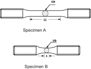
Test specimens were made with “V” joint for 1.4093 steel and with “X” joint for Armox 500T, as shown in Figure 1 . Dimension ratios for C1 specimens (steel 1.4903) are 8/10 = 0.8, and for P1 specimens (Armox 500T) are 7.4/7.5 = 0.99, which is practically square. Different shapes of the specimen cross-sections and grooves are also used to find out eventual effects of welded joint geometry on the proposed formulas for stress evaluation.

Dimensions [mm] of the specimens for steel 1.4903 (C1) and for Armox 500T (P1).

Digital image correlation (DIC) is a powerful non-contact technique for measuring surface displacement/strain fields, [ 21 ]. Simple geometric shapes can be treated by 2D analysis, while more advanced, 3D analysis, should be used for more complex geometric shapes, including welded joints, as applied and presented in [ 22 , 23 , 24 ]. The force during the experiment was controlled by strain, with the rate 2 mm/min. Setup of the experiment with the position of cameras is shown in Figure 2 . Using DIC method with two cameras (3D deformation measurement) and the Aramis software (Version 2M, GOM GmbH, Braunschweig, Germany) the current cross-section area can be determined. Accuracy of this method for strain measurement is very high, in order of micrometers, so it is a suitable method for the experiment performed here.

Setting up an experiment with the position of the cameras and with the extensometer set.

Finite element method (FEM) is nowadays a widely accepted numerical tool to get stress and strain distribution for many engineering problems, including elastic-plastic analysis of welded joints, even in the presence of cracks, and for other complex problems, [ 25 , 26 ].

Here, 3D FEM is used to evaluate stress concentration. Mesh was made with 3D linear elements, C3D8, with 8 nodes, with decreasing size in the weld metal down to 0.4 × 0.2 mm, as shown in Figure 3 , where one example of meshes deformed in weld metal is given. One quarter of specimen was modeled due to two planes of symmetry and appropriate boundary conditions applied (one rotation and two translations fixed). Load is defined as the negative pressure, according to the force applied and remote cross-section. More detailed description is given in [ 20 ].

FE model of specimen P1-1 with deformed weld metal.

Typical result for strain measurement by DIC is shown in Figure 4 , as obtained by the post-processing, using software Aramis.

Analysis of changes in the characteristic dimensions of the specimen C1-1.

The current cross-section area of the specimen was calculated using data obtained by Aramis, as shown in Figure 5 for specimen P1-1. One of the sides was actually measured, the opposite one taken as the mirror image, and two remaining are obtained by rotating the measured one for 90° and −90°.

Initial (marked by line) and final (green) cross-section area of specimen P1-1.

Figure 6 shows three stress–strain diagrams for both specimens, types C1 and P1, including engineering diagram, obtained by standard tensile test, marked in black. Remaining two diagrams represent true stress–strain curves, one determined according to Equations (1) and (2), marked in red, and the other one determined using measured cross-section areas of the specimen by DIC, marked in blue. One can see that the true stress is increased, if contraction measured by DIC ( Figure 5 ) is taken as relevant. This is why red curves in Figure 6 are marked as “true” and blue ones as true.

Comparison of true and engineering diagrams calculated by DIC method.

Results of FEM calculation are shown in Figure 7 for specimen C1-1 as an example of the procedure applied. Results for C1-1 specimen, with deformed weld metal according to strains and contraction obtained by DIC, show equivalent stress distribution, Figure 7 a, and normal stresses distribution, Figure 7 b, for the applied load 4 KN, producing remote tensile stress 100 MPa in the narrow part of the specimen, away from the welded joint area.

Stress distribution in specimen C1-1 with deformed weld metal: ( a ) equivalent stresses, ( b ) normal stresses, given in MPa.

From Figure 7 it can be concluded that the difference between maximum Misses equivalent stress and maximum normal stress is just 3.91 MPa (215.9–212 MPa) or 1.84%. This leads to the conclusion that the equivalent stress is not the dominant parameter for stress increase, but it is rather the stress concentration due to contraction. To calculate the actual stress with the stress concentration taken into account, the authors propose the following equations:

where C NM is the stress concentration factor and σ T is calculated as:

Stress concentration factor C NM can be separated into two factors, as follows:

where C zs takes into account the welded joint geometry and C EP stands for reduction of thickness. According to [ 22 ], C zs can be expressed for point 1, as follows:

where b 1 and R 1 are defined in Figure 8 for two characteristic points in a weld metal, together with their counterparts, b 2 and R 2 , used for calculating C zs for point 2.

Characteristic dimensions of weld metals: ( a ) V shape, ( b ) X shape.

Likewise, C EP can be defined as, [ 22 ]:

where t 0 and W 0 are initial values of thickness t and width W , Figure 8 . Therefore, the final expression for the stress concentration factor is:

The current cross-sectional area of the specimen ( A current ) was calculated using the data obtained by the DIC.

In the further analysis, numerical verification of coefficients for specimens C1-1 and P1-1 is shown for strains immediately before the fracture:

• Specimen C1-1
• Specimen P1-1

The values obtained in ABAQUS for the quarter of the specimen C1-1 and P1-1 at the characteristic points (1 and 2) are shown in Figure 9 . Stress for specimen C1-1, the maximum equivalent stresses (von Misses) are:

Maximum equivalent stresses in MPa at the characteristic points for specimens: ( a ) C1-1, ( b ) P1-1.

For specimen P1-1, the maximum equivalent stresses (Misses) by Abaqus are:

The equivalent stress values, obtained by ABAQUS and the stresses calculated by the formulas (10)–(15), are given in Table 5 . One should notice difference between stress values in points 1 and 2 for specimen C1-1 and almost the same stress values in these two points for specimen P1-1.

Comparison of the maximal stresses for the specimen C1-1 and P1-1.

In Figure 10 and Figure 11 , actual, true, and engineering stress–strain diagrams are presented for the specimen C1-1 and for the specimen P1-1, respectively.

Actual stress–strain diagrams for the specimen C1-1.

Actual stress–strain diagrams for the specimen P1-1.

4. Discussion

In this research the new methodology for true stress–strain curves are applied to undermatched welded joints made of different base metals, with different geometries (cross section and groove shape). One should notice that both base metals, used in this research, are low plasticity materials, especially Armox 500T (elongation A = 8%). Therefore, using only Equations (1) and (2) for determining the true stress–strain diagram produced questionable result, since the force drop is followed by the stress drop, as shown in Figure 6 for both base metals. Thus, the real contraction, as measured by 3D DIC, should be also taken into account, providing more realistic true stress–strain curves for both base metals, also shown in Figure 6 . As already mentioned, at this stage of development, one side of the specimen was actually measured, and the opposite one taken as the mirror image, while the remaining two sides are obtained by rotation. Anyhow, this issue will be tackled in future work by using at least four cameras to measure the two sides, and get the other two as mirror images. Measuring all the sides is probably too complicated, but it will be considered, as well.

Anyhow, in addition to previous, stress concentration due to geometry change should also be taken into account. Toward this end, new analytical expressions, i.e., formulas (10)–(15) have been introduced in the scope of this research, and verified by using the FEM. This was enabled by using results for strains and contraction, as obtained by DIC, to form FE models with different geometries of weld metal for different load levels, as explained in more detail in [ 20 ] using one base metal and one welded joint geometry. Here, this methodology is applied to both base metal and welded joint geometries to investigate eventual effects on actual stress–strain curves.

From Figure 10 and Figure 11 one can see that actual stresses σ max 1 actual and σ max 2 actual differ in specimen C1-1, while in the specimen P1-1 they are almost the same. Clearly, this is the effect of joint shape, since V joint (specimen C1-1) has different dimensions b 1 and b 2 , and thus different radii of curvature R 1 and R 2 , leading to different stress concentration factors, as well. For the specimen P1-1, difference between σ max 1 actual and σ max 2 actual is negligible due to the symmetry of joint shape (X), having approximately same values of b 1 and b 2 , and radii of curvature, R 1 and R 2 , leading to almost the same stress concentration factors.

It is also important to notice that differences in stresses calculated by the proposed formulas (10)–(15) and equivalent stresses obtained by Abaqus for the moment immediately before the fracture, Figure 9 , do not exceed 4.10% (specimen C1-1, Table 5 ). With this in mind, it can be considered that the proposed formulas evaluate the actual stress correctly for different levels of undermatching and different types of weld groove, as well as different shape ratio of the specimen cross section. Therefore, it was proved here that the proposed methodology is a general one, and can be applied to different materials and welded joint geometries.

One should notice that these effects are important for undermatched welded joints, since only in this case plastic strain and stress concentration develop in the weld metal, contrary to the overmatching welded joint, where they shift to the base metal, i.e., out of the critical zones of welded joint. Anyhow, it is still important to analyze overmatching effect in future research, since it is the most often case in practice.

5. Conclusions

The proposed Equations (10)–(15) proved to be sound basis to determine the actual stress–strain diagrams for undermatching the welded joints made of different base metals with different welded joint geometries. Actual stresses obtained by these formulas are in good agreement with the equivalent stresses obtained by Abaqus using finite element meshes constructed according to the geometry obtained by DIC.

It can be concluded that the actual value of the tensile strength of a welded joint is far above the value obtained by the standard tensile testing, presented by engineering stress–strain curves. This difference is a consequence of cross-section contraction and stress concentration in the most deformed zone, being the weld metal in the case of undermatched welded joint.

Cross-section contraction turned out to be an important factor in the case of low plasticity material, as used in this research, since the usual formulas for “true” stress–strain curves provide questionable behavior with drop of stress after maximum tensile force is reached.

The differences in normal and equivalent stress in rectangular specimens are not significant, leading to the conclusion that the dominant effect in rectangular specimens is not triaxial stress state, but the stress concentration due to contraction.

Further analysis should use more ductile material to analyze their behavior with respect to cross-section contraction and stress concentration, as well as other types of welded joints, such as overmatching joints and different welded joint geometries, to suggest eventual corrections to the proposed formulas.

Author Contributions

Conceptualization, N.Z.M. and A.S.S.; methodology, N.Z.M.; software, N.Z.M. and M.M.; validation, N.Z.M., A.S.S. and G.M.B.; formal analysis, N.Z.M. and A.S.S.; investigation, N.Z.M.; resources, V.L., M.M. and G.M.; data curation, N.Z.M., A.S.S.; writing—original draft preparation, N.Z.M.; writing—review and editing, A.S.S. and N.Z.M.; visualization, N.Z.M., A.S.S. and A.M.; supervision, A.S.S. and G.M.B. All authors have read and agreed to the published version of the manuscript.

The results presented are part of a research supported by MESTD RS by contract 451-03-9/2021-14/200105.

Institutional Review Board Statement

Not applicable.

Informed Consent Statement

Data availability statement, conflicts of interest.

The authors declare no conflict of interest.

Publisher’s Note: MDPI stays neutral with regard to jurisdictional claims in published maps and institutional affiliations.

• Architecture and Design
• Asian and Pacific Studies
• Business and Economics
• Classical and Ancient Near Eastern Studies
• Computer Sciences
• Cultural Studies
• Engineering
• General Interest
• Geosciences
• Industrial Chemistry
• Islamic and Middle Eastern Studies
• Jewish Studies
• Library and Information Science, Book Studies
• Life Sciences
• Linguistics and Semiotics
• Literary Studies
• Materials Sciences
• Mathematics
• Social Sciences
• Sports and Recreation
• Theology and Religion
• Publish your article
• The role of authors
• Promoting your article
• Abstracting & indexing
• Publishing Ethics
• Why publish with De Gruyter
• How to publish with De Gruyter
• Our book series
• Our subject areas
• Your digital product at De Gruyter
• Contribute to our reference works
• Product information
• Tools & resources
• Product Information
• Promotional Materials
• Orders and Inquiries
• FAQ for Library Suppliers and Book Sellers
• Repository Policy
• Free access policy
• Open Access agreements
• Database portals
• For Authors
• Customer service
• People + Culture
• Journal Management
• How to join us
• Working at De Gruyter
• Mission & Vision
• De Gruyter Foundation
• De Gruyter Ebound
• Our Responsibility
• Partner publishers

Your purchase has been completed. Your documents are now available to view.

Stress-strain curve of paper revisited

We have investigated a relation between micromechanical processes and the stress-strain curve of a dry fiber network during tensile loading. By using a detailed particle-level simulation tool we investigate, among other things, the impact of “non-traditional” bonding parameters, such as compliance of bonding regions, work of separation and the actual number of effective bonds. This is probably the first three-dimensional model which is capable of simulating the fracture process of paper accounting for nonlinearities at the fiber level and bond failures. The failure behavior of the network considered in the study could be changed significantly by relatively small changes in bond strength, as compared to the scatter in bonding data found in the literature. We have identified that compliance of the bonding regions has a significant impact on network strength. By comparing networks with weak and strong bonds, we concluded that large local strains are the precursors of bond failures and not the other way around.

© 2018 by Walter de Gruyter Berlin/Boston

• X / Twitter

Supplementary Materials

Please login or register with De Gruyter to order this product.

Journal and Issue

Articles in the same issue.

Advertisement

Stress-strain curve prediction of steel HAZ based on hardness

• Research Paper
• Published: 13 October 2021
• Volume 66 , pages 273–285, ( 2022 )

Cite this article

• T. Kasuya   ORCID: orcid.org/0000-0002-3303-0770 1 ,
• M. Inomoto 2 ,
• Y. Okazaki 2 ,
• S. Aihara 1 &
• M. Enoki 1  

431 Accesses

2 Citations

Explore all metrics

The prediction of the stress-strain curve at each point in steel HAZ (heat-affected zone) is rather complicated since the HAZ microstructure consists of multiple phases and varies continuously, and hence a simpler prediction method is desired. In this work, thermal simulation tests were conducted for tensile tests and hardness measurements. And using the experimental data, empirical equations to predict the stress-strain curve based on hardness have been developed. The stress-strain curve is divided into three regions. In the first region, the curve is described as a straight line. The curve in the second and the third regions is described by the Swift law, but the constants of the Swift law are different in the second and the third regions. The hardness value is the only data needed for the present prediction. The comparisons of the predictions with the experiments show that the present model can predict the stress-strain curves within an error of 100 MPa for most cases as long as the steel strength is up to 980 MPa. Hence, the present model can provide useful information for the evaluation of weld joint qualities.

This is a preview of subscription content, log in via an institution to check access.

Access this article

Price includes VAT (Russian Federation)

Instant access to the full article PDF.

Rent this article via DeepDyve

Institutional subscriptions

Similar content being viewed by others

Numerical prediction and experimental validation of forming limit curves of laminated half-hard aluminum sheets

Khalid Bouziane, Iliass EL Mrabti, … Nabil Moujibi

Residual Stress and Distortion during Quench Hardening of Steels: A Review

Augustine Samuel & K. Narayan Prabhu

Residual stress analysis in industrial parts: a comprehensive comparison of XRD methods

Ardeshir Sarmast, Jan Schubnell, … Eva Carl

Swift HW (1952) Plastic instability under plane stress. J Mech Phys Solids 1:1–18. https://doi.org/10.1016/0022-5096(52)90002-1

Article   Google Scholar  

Tomota Y, Umemoto M, Komatsubara N, Hiramatsu A, Nakazima N, Moriya A, Watanabe T, Nanba S, Anan G, Kunishige K, Higo Y, Miyahara M (1992) Prediction of mechanical properties of multi-phase steels based on stress-strain curves. ISIJ Int 32:343–349. https://doi.org/10.2355/isijinternational.32.343

Article   CAS   Google Scholar  

Rauch GC, Leslie WC (1972) The extent and nature of the strength-differential effect in steels. Metall Trans 3:373–385. https://doi.org/10.1007/BF02642041

Fernandes JV, Rodrigues DM, Menezes LF, Vieira MF (1998) A modified Swift law for prestrained materials. Int J Plast 14:537–550. https://doi.org/10.1016/S0749-6419(98)00027-8

Li L, Nagai K, Yin F (2010) Prediction on nominal stress-strain curve of anisotropic polycrystal with texture by FE analysis. Mater Trans 51:1825–1832. https://doi.org/10.2320/matertrans.M2010094

Dimatteo A, Colla V, Lovicu G, Valentini R (2015) Strain hardening behaviour prediction model for automotive high strength multiphase steels. Steel Res Int 86:1574–1582. https://doi.org/10.1002/srin.201400544

Tsuchida N, Harjo S, Ohnuki T, Tomota Y (2014) Stress-strain curves of steels. Tetsu-to-Haganẻ 100:1191–1206. https://doi.org/10.2355/tetsutohagane.100.1191 ( (in Japanese) )

Hill R (1965) Continuum micro-mechanics of elastoplastic polycrystals. J Mech Phys Solids 13:89–101. https://doi.org/10.1016/0022-5096(65)90023-2

Berveiller M, Zaoui A (1978) An extension of the self-consistent scheme to plastically-flowing polycrystals. J Mech Phys Solids 26:325–344. https://doi.org/10.1016/0022-5096(78)90003-0

Clausen B, Lorentzen T, Leffers T (1998) Self-consistent modelling of the deformation of F. C. C. polycrystals and its implications for diffraction measurements of internal stresses. Acta Mater 46:3087–3098. https://doi.org/10.1016/S1359-6454(98)00014-7

Weng GJ (1985) Micromechanical determination of two-phase plasticity. Int J Plast 1:275–287. https://doi.org/10.1016/0749-6419(85)90008-7

Weng GJ (1990) The overall elastoplastic stress-strain relations of dual-phase metals. J Mech Phys Solids 38:419–441. https://doi.org/10.1016/0022-5096(90)90007-Q

Matsuda K (2002) Prediction of stress-strain curves of elastic-plastic materials based on the Vickers indentation. Philos Mag A 82:1941–1951. https://doi.org/10.1080/01418610208235706

Itakura N, Yasuda K, Aoki M (1998) Properties of HT980 steel plates and welding materials with low cold cracking susceptibility and their applicability to penstocks. Kawasaki Steel Giho 30:174–180 (in Japanese) https://www.jfe-steel.co.jp/archives/ksc_giho/30-3/j30-174-180.pdf

CAS   Google Scholar  

Japanese Industrial Standard JIS G 4051 (2016) Carbon steels for machine structural use, Japanese Standard Association.

Japanese Industrial Standard JIS Z 2241 (2011) Metallic materials -tensile testing- method of test at room temperature, Japanese Standard Association.

Kasuya T, Inomoto M, Okazaki Y, Aihara S, Enoki M (2021) HAZ hardness prediction of boron-added steels. Weld World 65:1609–1621. https://doi.org/10.1007/s40194-021-01111-5

Kunigata M, Aihara S, Kawabata T, Kasuya T, Okazaki Y, Inomoto M (2020) Prediction of charpy impact toughness of steel weld heat-affected zones by combined micromechanics and stochastic fracture model -Part I: Model presentation. Eng Frac Mech 230:106965. https://doi.org/10.1016/j.engfracmech.2020.106965

Kunigata M, Aihara S, Kawabata T, Kasuya T, Okazaki Y, Inomoto M (2020) Prediction of charpy impact toughness of steel weld heat-affected zones by combined micromechanics and stochastic fracture model -Part II: Model validation by experiment. Eng Frac Mech 230:106966. https://doi.org/10.1016/j.engfracmech.2020.106966

Kasuya T, Yokobori AT, Ozeki G, Ohmi T, Enoki M (2021) Modelling of hydrogen diffusion in a weld cold cracking test: Part 1. Experimental determination of apparent diffusion coefficient and boundary condition. ISIJ Int 61:1245–1253. https://doi.org/10.2355/isijinternational.ISIJINT-2020-523

Kasuya T, Yokobori AT, Ozeki G, Ohmi T, Enoki M (2021) Modelling of hydrogen diffusion in a weld cold cracking test: Part 2. Numerical calculations. ISIJ Int 61:1254–1263. https://doi.org/10.2355/isijinternational.ISIJINT-2020-524

Download references

This work was partially supported by Council for Science, Technology and Innovation (CSTI), Cross-ministerial Strategic Innovation Promotion Program (SIP), “Structural Materials for Innovation” (Funding agency: JST), Japan.

Author information

Authors and affiliations.

Department of Materials Engineering, School of Engineering, The University of Tokyo, 7-3-1, Hongo, Bunkyoku, Tokyo, 133-8654, Japan

T. Kasuya, S. Aihara & M. Enoki

Materials Research Laboratory, Technical Development Group, KOBE STEEL, Ltd, 5-5, Takatsukadai 1-chome, Nishi-ku, Kobe, Hyogo, 651-2271, Japan

M. Inomoto & Y. Okazaki

You can also search for this author in PubMed   Google Scholar

Corresponding author

Correspondence to T. Kasuya .

Additional information

Publisher’s note.

Springer Nature remains neutral with regard to jurisdictional claims in published maps and institutional affiliations.

Recommended for publication by Commission IX - Behaviour of Metals Subjected to Welding

Rights and permissions

Reprints and permissions

About this article

Kasuya, T., Inomoto, M., Okazaki, Y. et al. Stress-strain curve prediction of steel HAZ based on hardness. Weld World 66 , 273–285 (2022). https://doi.org/10.1007/s40194-021-01198-w

Download citation

Received : 02 September 2021

Accepted : 01 October 2021

Published : 13 October 2021

Issue Date : February 2022

DOI : https://doi.org/10.1007/s40194-021-01198-w

Share this article

Anyone you share the following link with will be able to read this content:

Sorry, a shareable link is not currently available for this article.

Provided by the Springer Nature SharedIt content-sharing initiative

• Stress-strain curve
• Find a journal
• Publish with us
• Track your research

Plastic 3D Printing Service

Fused Deposition Modeling

HP Multi Jet Fusion

Selective Laser Sintering

Stereolithography

Production Photopolymers

Nexa3D LSPc

Direct Metal Laser Sintering

Metal Binder Jetting

Vapor Smoothing 3D Prints

CNC Machining

CNC Milling

CNC Turning

Wire EDM Machining

Medical CNC

CNC Routing

Sheet Metal Fabrication

Sheet Cutting

Laser Cutting

Waterjet Cutting

Plasma Cutting

Tube Bending

Laser Tube Cutting

Laser Engraving

Custom Die Cutting

Plastic Injection Molding

Quick-Turn Molding

Prototype Molding

Bridge Molding

Production Molding

Overmolding

Insert Molding

Urethane and Silicone Casting

Plastic Extrusion

HDPE Injection Molding

Injection Molded Surface Finishes

Custom Plastic Fabrication

Micro Molding

Metal Injection Molding

Die Casting

Metal Stamping

Metal Extrusion

Custom Hydroforming

Assembly Services

Rapid Prototyping

High-Volume Production

Precision Grinding

Surface Grinding

Powder Coating

Aerospace and Defense

Consumer Products

Design Services

Electronics and Semiconductors

Hardware Startups

Medical and Dental

Supply Chain and Purchasing

All Technical Guides

Design Guides

eBooks Library

3D Printing Articles

Injection Molding Articles

Machining Articles

Sheet Cutting Articles

Xometry Production Guide

CAD Add-ins

Manufacturing Standards

Standard Sheet Thicknesses

Standard Tube and Pipe Sizes

Standard Threads

Standard Inserts

ITAR and Certifications

Case Studies

Supplier Community

Release Notes

Call: +1-800-983-1959

Email: [email protected]

Discover Xometry Teamspace

Meet An Account Rep

eProcurement Integrations

Bulk Upload for Production Quotes

Onboard Xometry As Your Vendor

How to Use the Xometry Instant Quoting Engine®

Test Drive Xometry

Xometry’s Quality Assurance

Xometry’s Supplier Network

Xometry's Machine Learning

Part Revisions & Same-Suppliers for Repeat Orders

Xometry's Privacy and Security

Xometry's Injection Molding Service

What Is Stress-Strain Curve?

Learn more about how a stress-strain curve helps determine a material's behavior.

A stress-strain curve is a graphical depiction of a material’s behavior when subjected to increasing loads. Stress is defined as the ratio of force to cross-sectional area, while strain is defined as the ratio of the change in length of a dimension to the dimension’s original length. Stress-strain curves can be generated to investigate a material’s behavior when any type of load (tensile, compression, shear, bending, torsion) is applied. We will, however, will focus solely on the stress-strain curves generated by tensile loads. Stress-strain curves generated for tensile loads are important because they enable engineers to quickly determine several mechanical properties of a material including: modulus of elasticity (Young’s modulus), yield strength, ultimate strength, and ductility. A stress-strain curve is obtained by conducting a tensile test (a type of test where a load is continuously applied to a test specimen until it fractures). The stress experienced by the part is graphed on the Y-axis, while the strain is graphed on the X-axis. This article will define the stress-strain curve, its different regions, how to interpret it, and its importance to material selection.

.css-2xf3ee{font-size:0.6em;margin-left:-2em;position:absolute;color:#22445F;} .css-14nvrlq{display:inline-block;line-height:1;height:1em;background-color:currentColor;-webkit-mask:url(https://assets.xometry.com/fontawesome-pro/v6/svgs/light/link.svg) no-repeat center/contain content-box;mask:url(https://assets.xometry.com/fontawesome-pro/v6/svgs/light/link.svg) no-repeat center/contain content-box;-webkit-mask:url(https://assets.xometry.com/fontawesome-pro/v6/svgs/light/link.svg) no-repeat center/contain content-box;aspect-ratio:640/512;vertical-align:-15%;}.css-14nvrlq:before{content:"";} What Is Stress?

Stress is the amount of force applied to a cross-sectional area. It’s a highly important calculation because it allows engineers to quantify the amount of force that a material can tolerate before fracturing. This parameter is used by engineers to select materials and designs that will result in safe, durable structures. The formula for stress is shown below:

Stress formula.

• 𝜎 is the stress
• F is the applied force
• A is the cross-sectional area. 

The SI unit for stress is the Pascal (Pa), but pounds per square inch (psi) is also commonly used.

What Is Strain?

Strain is defined as the deformation experienced by a material relative to its original dimensions. Strain, like stress, is an essential calculation because it helps engineers quantify how much deformation a material can accommodate before it permanently deforms or fractures. The formula for strain is defined below: 

Strain formula.

• ε is the strain
• Lf is the final length
•  L0 is the initial length

Strain is a unitless value since the numbers in both the top and bottom of the formula are in units of length.

Why Is Stress-Strain Curve Important?

The stress-strain curve is important because it allows engineers to quickly determine several of the most critical and fundamental mechanical properties of any material. A single tensile test can produce a stress-strain graph, which then allows the following properties of a material to be obtained:

• Young’s modulus
• Yield strength
• Ultimate tensile strength
• Poisson’s ratio

How Is the Stress-Strain Curve Measured?

Stress-strain curves are generated automatically by modern tensile testing machines. These machines continuously monitor and record the force applied to a test specimen and the amount of deformation it experiences as a result of that load. The most commonly used test methods for tensile testing and creating standardized stress-strain curves are those issued by ASTM International. ASTM E8 standardizes tensile tests for metallic materials while ASTM D638 standardizes tensile tests for plastic materials. The steps to creating a stress-strain curve are described in the list below:

• Prepare the test specimen to the required dimensions.
• Mount the test specimen in the jaws of the tensile testing machine.
• Apply a continuously increasing tensile load to the specimen until it breaks.
• The tensile testing machine will record the stress and strain experienced by the test specimen based on readings of force applied by the load cell and displacement of the jaws holding the test piece.

What Are the Different Stress-Strains?

There are two types of stresses and strains that are described in detail below:

1. Engineering Stress and Strain

Engineering stress and strain are the stress-strain values of material calculated without accounting for the fine details of plastic deformation. These values are also referred to as nominal stress and strain. The values for engineering stress and strain are convenient for measuring the performance of a material and can be directly obtained from a standard tensile test. The formula for engineering stress is shown below:

Engineering stress formula.

Where A0 is the original cross-sectional area of the test specimen. The SI unit for stress is the Pascal (Pa), but pounds per square inch (psi) is also commonly used. 

The formula for engineering strain is given below:

Engineering strain formula.

Strain is a unitless measurement.

2. True Stress and Strain

True stress and strain are the actual stress and strain experienced by a material while taking into account its deformation during a tensile test. It is ideal for analyzing the mechanical properties of a material. True stress and strain must be calculated from experimental data related to the test specimen’s instantaneous gauge length, cross-section area, and applied load throughout the test. The formula for true stress is shown below:

True stress formula.

Where Ai is the instantaneous cross-sectional area. The formula for true strain is shown below:

True strain formula.

Where Li is the instantaneous length.

What Are the Stages of the Stress-Strain Curve?

A stress-strain diagram has three stages. In the first stage, the material experiences only elastic deformation. When the applied stress is released, the material returns to its original dimensions. 

Uniform plastic deformation takes place in the second stage. This stage begins at the yield point and continues for as long as the material can continue to strengthen through strain hardening (the same process that occurs in cold forming) with every new increment of the applied load. Eventually, the material's capacity for stable plastic deformation is exhausted. The amount of plastic strain that can be tolerated during this phase tells us a lot about the material's relative brittleness or ductility.

The final stage of a tensile test is referred to as “necking.” This stage occurs after the material’s ultimate tensile stress is reached, and no further strain hardening is possible. Instead of continued, stable deformation, a region of localized deformation forms somewhere in the cross-section of the test specimen. The excessive tensile stresses reduce the material’s dimensions that are perpendicular to the applied force which causes a significant reduction in area. This makes the material have the shape of a “neck”. Once necking begins, the engineering stress of the material decreases while the true stress continues to increase.  The material fractures soon after necking begins.

How To Read the Stress-Strain Graph?

The general steps for how to read a stress-strain graph are described below:

• Pick a stress value on the Y-axis.
• Trace a horizontal line from the Y-axis until it intersects the stress-strain curve’s line. 
• Mark the point where the horizontal line and stress-strain curve line intersect.
• Trace a vertical line down from the intersection point to X-axis. The two traced lines should form a sharp, 90° corner.
• The stress value chosen from step 1 shows the stress that corresponds to the strain, or deformation, experienced by the test specimen at that point.

The steps above can be used to determine the strain experienced by the test specimen at the moments the yield stress, ultimate tensile strength, and fracture point are reached.

What Are the Different Regions of the Stress-Strain Curve Graph?

Five significant points can easily be picked off a stress-strain curve. The interpretation of each point offers unique insight into the mechanical behavior of a material. The five points are described in detail below:

1. Proportional Limit

The proportional limit refers to the point at the end of the linear portion of the stress-strain curve.All of the deformation up to the proportional limit occurs with one proportionality constant, called Young's modulus. It is calculated as the slope of the line (stress divided by strain) up to the proportional limit. In this region, Young’s modulus can be obtained by calculating the slope of the line. 

2. Elastic Limit

The elastic limit is the observed point on the stress-strain curve where elastic deformation ends and plastic deformation begins. When the applied load is released at any point up to the elastic limit, the material will regain its starting dimensions. In metals, the elastic limit is often difficult to distinguish from the proportional limit and the yield point since the points on the curve are so close to each other. Therefore, the elastic limit is more often used for educational purposes rather than actual characterization of a material’s properties.

3. Yield Point

The yield point is similar to the elastic limit of the stress-strain curve in that it also describes the point where elastic deformation ends and plastic deformation begins. The primary difference between the two is that the yield point is a calculated value that precisely describes the elastic limit, or yield strength of the material. The yield point is determined by offsetting the linear portion of the stress-strain curve by +0.2% along the horizontal (strain) axis. The intersection point of the offset line with the original stress-strain curve is considered the yield strength of the material.

4. Ultimate Stress Point

The ultimate stress point, or ultimate tensile strength, is the highest stress observed on the stress-strain curve. After the ultimate tensile strength is reached, the test specimen begins to “neck.” It’s important to note that while the ultimate stress point is the highest point observed on the stress-strain curve, the actual highest stress is actually the true stress at fracture.

5. Fracture or Breaking Point 

The fracture or breaking point is the point on the stress-strain curve where the test specimen has deformed so much that its microstructure gives and the part fractures.

How To Make a Stress-Strain Curve?

A stress-strain curve is made by conducting a tensile test using a universal testing machine. The testing machine will automatically capture the data to produce a stress-strain curve as the load increases and the specimen deforms. 

What Is the Use of the Stress-Strain Graph?

The stress-strain graph is used to determine various mechanical properties of a material, including elastic modulus, Poisson’s ratio, yield stress, and ultimate tensile strength. These properties help engineers select materials for applications where load-bearing capability is critical.

What Is the Stress-Strain Curve of a Ductile Material? 

Figure 1 below is an example of a stress-strain curve of a ductile and brittle material:

Stress-strain curves of a ductile and a brittle material.

Image Credit: https://www.researchgate.net/

What Is the Stress-Strain Curve of a Brittle Material?

The stress-strain curve of a brittle material is a steeply sloped line that shows the stress increasing rapidly with little strain. Unlike ductile materials, the stress-strain curve for a brittle material shows little plastic deformation after the yield stress (yield point) is reached. The material fractures soon after the yield stress.  Figure 1 above is an example of a stress-strain curve of brittle material.

What Is the Difference Between Engineering Stress-Strain and True Stress-Strain?

The differences between engineering stress-strain and true stress-strain are listed below: 

• Engineering stress-strain doesn’t take into account the material’s deformation while true stress-strain does.
• Engineering strain is the ratio of the change in length to the original length while a true strain is the natural logarithm of the instantaneous length over the original length.
• Engineering stress-strain is ideal for determining material performance while true stress-strain is ideal for determining material properties.

What Is the Difference Between Stress and Strain?

The differences between stress and strain are listed below:

• Stress is the force per unit area, while a strain is a variation in the length of a dimension over the original length of the dimension.
• Stress has units of Pa or psi while a strain is unitless.
• The symbol for stress is 𝛔 while the symbol for strain is 𝞊.
• Stress is required to cause strain.
• Stress cannot be directly measured and is calculated through mathematical relations while a strain can be directly measured.

Xometry provides a wide range of manufacturing capabilities, including 3D printing and other value-added services for all of your prototyping and production needs. Visit our website to learn more or to request a free, no-obligation quote .

The content appearing on this webpage is for informational purposes only. Xometry makes no representation or warranty of any kind, be it expressed or implied, as to the accuracy, completeness, or validity of the information. Any performance parameters, geometric tolerances, specific design features, quality and types of materials, or processes should not be inferred to represent what will be delivered by third-party suppliers or manufacturers through Xometry’s network. Buyers seeking quotes for parts are responsible for defining the specific requirements for those parts. Please refer to our terms and conditions for more information.