project cost estimation case study

• Contact sales

Start free trial

Project Cost Estimation: How to Estimate Project Cost

Good cost estimation is essential for project management success. Many costs can appear over the project management life cycle, and an accurate project cost estimation method can be the difference between a successful plan and a failed one. Project cost estimating, however, is easier said than done. Projects bring risks, and risks bring unexpected costs and cost management issues.

What Is Project Cost Estimation?

Project cost estimation is the process that takes direct costs, indirect costs and other types of project costs into account and calculates a budget that meets the financial commitment necessary for a successful project. To do this, project managers and project estimators use a cost breakdown structure to determine all the costs in a project.

Project cost estimation is critical for any type of project , from building a bridge to developing that new killer app. Everything costs money, so the clearer you are on the amount required, the more likely you and your project team will achieve your objective.

Project cost estimating is a critical step during the project planning phase because it helps project managers create a project budget that covers the project costs that are needed to achieve the goals and objectives of the project set forth by executives and project stakeholders.

Get your free

Project Estimate Template

Use this free Project Estimate Template for Excel to manage your projects better.

What Is a Project Estimate?

A project estimate is the process of accurately forecasting the time, cost and resources required for a project. This is done by looking at historical data, getting information from the client and itemizing each resource and its duration of use in the project.

To create a project estimate, you should first define your project scope and then create a project cost breakdown structure, which allows you to pinpoint all of your different project costs for each stage of the project life cycle.

Project cost estimation is simplified with the help of project management software like ProjectManager . Add project budgets and planned costs for specific tasks and include labor rates for your team. When you build your plan on our Gantt chart, your estimated project costs will calculate automatically. Plus, as the project unfolds, you can track your costs in real time on our automated dashboard. Try it for free today.

What Is a Project Cost Breakdown Structure?

A cost breakdown structure (CBS) is a very important project costing tool that details the individual costs of a project on a document. Similar to a work breakdown structure (WBS) , it’s a hierarchical chart where each row represents a type of cost or item. This is done at the task level, which is called a bottom-up analysis.

Creating a cost breakdown structure might be time-consuming, but one that’s worth the effort in that the result is a more accurate estimate of costs than you’d get with a top-down approach, such as basing all your estimates on the costs of previous, similar projects.

Using a cost breakdown structure is an essential part of project cost management and resource management . By zeroing in on costs at the task level early during the project planning phase, you’re less likely to miss hidden costs that could come up later during the project execution stage and throw your project budget off.

Types of Project Costs

There are five main types of costs that make up your total project cost. Here’s a quick overview of these types of project costs and how to measure them.

• Direct costs: Direct costs are those that occur in a project and are attached to specific activities. These are generally costs that are easier to accurately estimate. They include raw materials, labor, supplies, etc.
• Indirect costs: Indirect costs in a project are those that are in support of the project, such as administrative fees. These can include everything from rent to salaries of the administrative staff to utilities, etc.
• Fixed costs: Fixed costs, as the name suggests, are those that don’t change throughout the life cycle of a project . Some examples of fixed costs include setup costs, rental costs, insurance premiums, property taxes, etc.
• Variable costs: Variable costs are costs that change due to the amount of work that’s done in the project and are variable in nature. These costs can include hourly labor wages, materials, fuel costs and so on.
• Sunk costs: In project cost estimating, when an investment has already been incurred and can’t be recovered it’s called a sunk cost or retrospective cost. Some examples of sunk costs include marketing, research, installation of new software, etc.

What Does a Project Estimator Do?

The project estimator or cost estimator, is tasked with figuring out the duration of the project in order to deliver it successfully. This includes determining the resources needed, including labor, materials, etc., which informs the project budget .

In order to do this, a project estimator must understand the project and its phases and be able to research the historical data of projects that were similar and executed in the past. Cost estimators also need to have a firm grasp of mathematical concepts.

Unlike a project manager , who’s responsible for the delivery and oversight of the project, a project estimator is focused on the direct and indirect costs associated with the project. Project estimators work closely with contractual professionals to develop accurate estimates, which are presented to project leaders.

Project Cost Estimation Techniques

All of these factors impact project cost estimation, making it difficult to come up with precise estimates. Luckily, there are cost estimating techniques that can help with developing a more accurate cost estimation.

Analogous Estimating

Seek the help of experts who have experience in similar projects, or use your own historical data. If you have access to relevant historical data, try analogous estimating, which can show precedents that help define what your future costs will be in the early stages of the project.

Parametric Estimating

There’s statistical modeling or parametric estimating , another cost estimation method that also uses historical data of key cost drivers and then calculates what those costs would be if the duration or another of the project is changed.

Bottom-Up Estimating

A more granular approach is bottom-up estimating, which uses estimates of individual tasks and then adds those up to determine the overall cost of the project. This cost-estimating method is even more detailed than parametric estimating and is used in complex projects with many variables such as software development or construction projects.

Three-Point Estimate

Another approach is the three-point estimate, which comes up with three scenarios: most likely, optimistic and pessimistic ranges. These are then put into an equation to develop an estimation.

Reserve Analysis

Reserve analysis determines how much contingency reserve must be allocated. This cost estimation method tries to wrangle uncertainty.

Cost of Quality

Cost of quality uses money spent during the project to avoid failures and money applied after the project to address failures. This can help fine-tune your overall project cost estimation. Plus, comparing bids from vendors can also help figure out costs.

Dynamic Project Costing Tools

Whenever you’re estimating costs, it helps to use online software to collect all of your project information. Project management software can be used in Congress with many of these techniques to help facilitate the process. Use online software to define your project teams, tasks and goals. Even manage your vendors and track costs as the project unfolds. We’ll show you how.

Free Project Cost Estimation Template

ProjectManager has free templates for every aspect of managing a project, including a free cost estimate template for Excel. It can be used for any project by simply replacing the items in the description column with those items that are relevant to your project.

This free cost estimate template has all the fields you’d need to fill in when estimating project costs. For example, there’s the description column followed by the vendor or subcontractor column and then there are columns to capture the labor and raw materials costs. These can be added together by line and then a total project cost can be calculated by the template.

Naturally, a cost estimate template is a static document. It’s handy in terms of collecting all your project costs and tracking them over the life cycle of the project. However, all that data must be manually added, which takes time and effort—two things that you don’t have in abundance when managing a project. Once you’re ready to streamline the cost estimate process you’ll find that there are many project management software solutions that can build budgets and track them in real time to keep you from overspending.

How to Estimate Project Costs in 10 Steps

The U.S. government has identified a 10-step process that results in reliable and valid cost estimates for project management . Those steps are outlined below.

• Define the cost estimate’s purpose: Determine the purpose of the cost estimate, the level of detail that is required, who receives the estimate and the overall scope of the estimate.
• Develop an estimating plan: Assemble a cost-estimating team and outline their estimation techniques. Develop a timeline , and determine who will do the independent cost estimate. Finally, create the team’s schedule.
• Define characteristics: Create a baseline description of the purpose, system and performance characteristics. This includes any technology implications, system configurations, schedules, strategies and relations to existing systems. Don’t forget support, security, risk items, testing and production, deployment and maintenance and any similar legacy systems.
• Determine cost estimating techniques: Define a work breakdown structure (WBS) and choose an estimating method that’s best suited for each element in the WBS. Cross-check for cost and schedule drivers; then create a checklist.
• Identify rules, assumptions and obtain data: Clearly define what’s included and excluded from the estimate and identify specific assumptions.
• Develop a point estimate: Develop a cost model by estimating each WBS element.
• Conduct a sensitivity analysis: Test the sensitivity of costs to changes in estimating input values and key assumptions, and determine key cost drivers.
• Conduct risk and uncertainty analysis: Determine the cost, schedule and technical risks inherent with each item on the WBS and how to manage them.
• Document the estimate and present it to management: Having documentation for each step in the cost estimate process keeps everyone on the same page with the cost estimate. Then you can brief the project stakeholders on cost estimates to get their approval.
• Update the cost estimate: Any changes to the cost estimate must be updated and reported . Also, perform a postmortem where you can document lessons learned.

Project Cost Estimation Example

Let’s take a moment to create a hypothetical project and run through a general cost estimate example to see how this process works. Construction cost estimation is straightforward so we’ll use a construction estimate example. This construction project will focus on the general requirements for cost estimation in project management.

Related:  Construction Estimate Template

First, you’ll want to have a list describing the various elements needed to build your construction project. Gather all your construction project management documents such as plans, designs and specifications, blueprints and permits to find out cost data. In your documents, you’ll find administrative costs, financing costs, legal fees, engineering fees, insurance and other cost items.

Now it’s time to use a work breakdown structure (WBS) to identify all your construction project activities. Identify the labor costs, direct costs and indirect costs associated with every activity in your project schedule. There are various cost estimating techniques such as bottom-up estimating which allow contractors to estimate costs for each construction activity to create accurate proposals for the construction bidding process.

These costs are then added together for a line total, and those line totals are added together to determine your total project cost. Having a cost estimation template is a good tool to collect and track this information.

ProjectManager Helps With Project Cost Estimation

ProjectManager is a project management software that has features to help create a more accurate project cost estimate. Our Gantt chart can be used to help you track costs and expenditures for projects and tasks.

Estimate Costs of Specific Tasks

When estimating individual tasks, costs can also be collected and tracked on our online Gantt chart. Here you can add a column for the estimated costs, baseline cost and the actual costs to help you keep the project on budget once it’s been executed.

Our online Gantt chart can not only track tasks, but you can set it up to track materials and fixed costs associated with each project task and monitor the difference between budget and actual costs. All of this data is collected on one page.

Start by creating a project and then go to the Gantt view on ProjectManager. If you already have data, you can import it by clicking on the import button on the top right-hand side of the page. Or you can use this online Gantt chart to collect the data. It can be easily shared with team members and stakeholders when you’re ready to get input or approval.

Estimate Costs of Resources

The resource management feature on ProjectManager is another tool that can help you achieve a more accurate project cost estimate. It offers a way to look at your costs through the workload across tasks and projects.

When planning a project with our resource management tool , you can account for employee schedules, equipment rentals, holidays and office space, among other factors that’ll impact your budget. Distributing project resources is one way to balance a budget.

Create a resource plan by scheduling the dates for planned resources, how long you’ll need them and the people who will be involved. That includes any equipment or site rentals. Break that down into the number of resources needed for each activity on a daily basis and you’ll be able to create a schedule with detailed resources, including duration and estimated costs.

FAQs About Project Cost Estimation

Here are some of the most frequently asked questions about project cost estimation online.

What Is Project Cost Analysis?

A project cost analysis is used to determine the costs and benefits associated with a project. It’s a process used to determine if the project is feasible.

What Is a Project Cost Breakdown?

A project cost breakdown is the process by which a project manager estimates what will need to be spent in order to deliver a project. A cost breakdown structure is used during the project cost estimating process to ensure all costs are accounted for.

Why Is Project Cost Estimation Important?

Cost estimation and cost management are an essential part of project management. The project manager is responsible for making the most accurate project budget possible by using a cost breakdown structure and project estimating techniques.

The project budget collects indirect costs and direct costs as it estimates the overall cost of delivering the project on time and meeting quality expectations. That means, whatever you’re going to need to make the project a success will be thought through during the cost estimation process.

Related Content

• Project Estimation Techniques: A Quick Guide
• Time Estimation in Project Management: Tips & Techniques
• Calculating Estimate at Completion (EAC)
• Parametric Estimating In Project Management
• What Is Job Costing? When to Use a Costing Sheet (Example Included)

When estimating costs on a project, you want to have the best tools to help you calculate a more accurate budget. ProjectManager is online project management software with online Gantt charts and resource management features that give you control over your project costs. See how ProjectManager can assist with your project cost estimation by taking this free 30-day trial today.

Deliver your projects on time and under budget

Start planning your projects.

Estimating Cost of a Project: Techniques and Examples

Estimating cost is an important process in project management as it is the basis for determining and controlling the project budget. Costs are estimated for the first time at the beginning of a project or even before a project has started. Subsequently, the (re-)estimation of the project cost is repeated on an ongoing basis to account for more detailed information or changes to the scope or timeline.

For instance, if the earned value management measures that are used for controlling project cost indicate significant variances from the budget, a re-estimation of the cost and schedule and a revisiting of the overall budget can be inevitable.

The methods introduced in this article are tools and techniques of the “Estimate Costs” process that is part of PMI’s Knowledge Area “Project Cost Management” (see PMBOK®, 6 th edition, ch. 7.2).

What Is a Cost Estimate?

Rough order of magnitude vs. definitive estimate, estimate to complete (etc) and estimate at completion (eac), when are cost estimated, why is cost estimation important in project management, comparison of estimation techniques, expert judgment       , analogous estimating , parametric estimating, bottom-up estimating, three-point estimating.

A Cost estimate is a quantified expectation of how many resources are required to complete a project or parts of a project.

Such cost estimates are often expressed in currency units. However, other units such as man-days can also be used if the currency amounts are not applicable or irrelevant.

There are different types of cost estimates. The Project Management Body of Knowledge lists the rough order of magnitude (ROM) and the definitive estimate. Both types differ in respect of their accuracy, the project phases in which they are used as well as the available tools and techniques. Some projects use additional, sometimes industry-specific types of estimates.

Cost estimating involves different tools and techniques which typically include

• Expert judgment,
• Analogous estimating,
• Parametric estimating,
• Bottom-up estimating,
• Three-point estimating, and
• Cost of quality.

Read on to learn the details of these techniques, supplemented with examples and practical considerations.

What Are the Types of Cost Estimates?

According to the PMBOK®, there are 2 types of cost estimates:

• Rough order of magnitude (ROM) with an accuracy of -25% to + 75% (other frameworks quote a range of +/-50%) and
• Definitive estimate with an accuracy range of -5% to +10%.

Some sources also list so-called preliminary estimates and budget estimates as further gradations of estimate types. There are also industry-specific types of estimates such as design and bid estimates in construction projects ( source ). However, the current PMI project management framework only refers to the 2 above-mentioned types.

If the budget has to be revisited part way through a project, a so-called estimate to complete (ETC) is determined.

The obvious difference between these 2 types of estimates is the accuracy: the ROM is rather inaccurate with a broad range of possible outcomes. It is therefore typically used in project initiation phases where a ballpark figure is sufficient to get a project started.

The definitive estimate is determined in the course of the project when more information and resources for accurate estimates are available.

Read this article for more details on the ROM and the differences between ROM and definitive estimate .

If partway in a project it turns out that the budget baseline (based on previous estimates) cannot be met, a re-estimation of the project cost is required.

This is done by determining an estimate to complete (ETC) which is used to calculate a new estimate at completion (EAC) that replaces the initial budget at completion and thus becomes the new cost baseline of a project.

Costs are estimated at different points in time throughout the project. The PMBOK states that the process is performed “periodically throughout the project as needed” (source: PMBOK®, 6 th edition, ch. 7.2).

The first point to estimate cost is during the initiation phase, e.g. when the project business case or the project charter is created. For these documents, a project manager has to determine the amount of resources that is required to complete the project.

As the information that is available at that point is usually not very detailed, the project manager will likely end up producing a rough order of magnitude estimate rather than a definitive estimate. Later in the project when more information is available, this order of magnitude estimate will be replaced with a definitive estimate.

After the project initiation phase, the cost will be re-assessed during the planning phase, using the techniques introduced in this article.

In subsequent phases, costs are typically (re-)estimated if relevant new information and details become known or if changes to the project scope or timeline occur. One of the common reasons for re-estimating cost is, for instance, when the indicators of the project controlling suggest that the original budget baseline cannot be met.

Estimating costs is one of the core activities of project management and planning. This is because a project is defined as being subject to at least three fundamental constraints : scope , budget and time. Cost estimates are obviously addressing the budget constraint; hence they are highly relevant for the management of a project. The initial rough cost estimate is usually included in the project charter as well as in the business case of a project.

The estimation of costs is also necessary to compute the project budget which is subject to the approval of the project sponsor(s). In fact, the process “determine budget” uses a technique called “cost aggregation” which directly refers to the outputs of the “estimate cost” process.

Cost estimates are the basis for allocating budget to work packages and deliverables which can be politically sensitive within a project as well as among its stakeholders. Therefore, budget determination and assignment require some stakeholder involvement, communication and, in many cases, their approval.

In addition, cost estimates are input parameters for the earned value and variance analyses as well as forecasting of project costs .

Tools and Techniques for Estimating Project Cost

This section provides an overview of the tools and techniques for estimating project costs. These methods refer to chapter 7.2.2 of PMI’s Project Management Body of Knowledge .

Click on the links to the detailed articles on these techniques to find further explanations and practical examples.

This table compares the approaches to estimating project costs and highlights the differences between these techniques.

This technique is suggested by the PMBOK (ch. 4.1.2.1) as a way to produce a cost estimate.

If you or your team have experience with the kind of work that is in the scope of a project, you can use expert judgment to produce an estimate. This requires a certain level of familiarity with the subject of a project and its environments such as the industry and the organization.

Expert judgment can be applied to both bottom-up and top-down estimating. Its accuracy depends greatly on the number and experience of the experts involved, the clarity of the planned activities and steps as well as the type of the project.

Two examples of expert judgment are:

• Estimating the rough order of magnitude at the beginning of a project. At that time, estimates are often performed top-down due to a lack of team members. more accurate estimation techniques (such as parametric estimating) may also not be available due to a lack of data.
• (Re-)estimating the efforts needed to generate the deliverables of a work breakdown structure (WBS) by asking those responsible for work packages and activities to estimate their resource requirements. This type of expert judgment can lead to comparatively accurate results.

Besides being an estimation technique on its own, expert judgment is also inherent to the other estimation techniques. For instance, if the comparability of previous work and the current project is assessed or adjustments to parametric estimates are determined.

Analogous estimating refers to the use of observed cost figures and related values in previous projects (or portions of a project). In order to be accurate, the type and nature of these reference activities must be comparable with the current project.

“Analogous estimating, also called top-down estimating, is a form of expert judgment.” Source: Heldman, Kim. PMP: Project Management Professional Exam Study

This technique uses historical data in the form of values and parameters to determine the expected resource requirements of a current project. The historic values are adopted for the current work and can be adjusted for differences in scope or complexity. Analogous estimating is categorized as a gross value estimating approach.

In general, analogous estimates are used if a project has access to historical data on similar types of work while the details and resources for more accurate estimates in the current project, such as parametric or bottom-up estimating, are not available.

Parametric estimating is a statistical approach to determine the expected resource requirements. It is based on the assumed or proven relationship of parameters and values. Simple examples are the building cost per square foot in construction projects or the implementation cost per data field in IT projects.

If, for instance, the cost of implementing a new data field in an IT system were $20,000 according to historical data, and a project required 15 new data fields, the total cost of this part of the project would be 15 x $20,000 = $300,000.

The input data can be obtained from previous projects or external data sources such as industry benchmarks or publicly available statistics.

In practice, this technique is employed with a broad variety of sophistication and accuracy. It can be used with a simple ‘rule of three’ calculation but also in conjunction with a complex statistical or algorithmic model that may consider multiple quantitative and qualitative parameters for detailed regression analyses.

In projects that do not use an explicit statistical correlation analysis, some expert judgment is required to assess whether it would be reasonable to apply the historic parameters to the current project. Complexities of projects and activities vary and may therefore require certain adjustments.

For instance, building a highway in a mountainous region likely produces a higher cost per mile than in a flat area. IT development projects in complex IT architectures or systems tend to require more resources than a less complex environment.

Another consideration concerns the expertise and experience of the project team. If a previous project was delivered by highly skilled and experienced resources while the current team is just at the beginning of its learning curve, using unadjusted historic data may understate the estimated cost.

Similar to analogous estimates, adjustments can be made to adapt the parametric estimates to the current project.

Depending on the quality of the input data and its applicability to the current type of work, the parametric estimation technique can produce very accurate figures. However, the higher the accuracy desired the more resources are needed to perform the data gathering and statistical analyses.

Bottom-up estimation refers to a technique that involves estimating the cost at a granular level of work units. The estimates for all components of a project are then aggregated in order to determine the overall project cost estimate.

In practice, these estimates are often performed at the lowest level of the work breakdown structure (WBS), e.g. for work packages or even activities.

While there is no clear rule on who should be performing this estimation, it seems to be a good practice in project management: asking those project team members who are operationally in charge of the respective work packages or activities to estimate there on work.

Thus, this approach to estimating costs often comes with significantly higher accuracy than top-down estimations. However, obtaining and aggregating these granular estimates normally requires some resources and can potentially become a political challenge, especially in large or complex projects.

Three-point estimating is a technique that usually leverages on bottom-up estimates, analogous or expert estimates. The concept requires three different points of estimates: the optimistic (best case), pessimistic (worst case) and the most likely cost estimate.

Based on these 3 points, a weighted average cost estimate is determined that overweighs the “most likely” point. This can be done by assuming a triangular distribution, a PERT or beta distribution.

Read this article for further explanation and examples of this technique.

In this article, we have discussed the techniques of cost estimating as suggested by the PMBOK. Note that the level of detail and granularity of the estimates usually increases throughout the project.

In the initiation phase, the rough order of magnitude (ROM) is often the only type of estimate that can be obtained. Definitive estimates will usually require techniques such as analogous, bottom-up and parametric estimating that may only become available in later stages of a project.

Parametric and bottom-up estimates are usually the techniques that provide the most accurate cost projections. They are commonly used if the budget needs to be revisited and replaced with a new estimate at completion.

When a budget is determined and approved, earned value analysis and variance analysis help project managers control the cost and value generated in a project. You will find more details on the measures and the techniques in this article .

An empirical study on a single company’s cost estimations of 338 software projects

• Published: 25 November 2022
• Volume 28 , article number  11 , ( 2023 )

Cite this article

• Christian Schürhoff 1 ,
• Stefan Hanenberg   ORCID: orcid.org/0000-0001-5936-2143 1 &
• Volker Gruhn 1  

355 Accesses

10 Altmetric

Explore all metrics

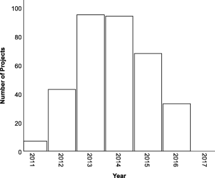
A recurring statement in the literature is that cost estimations in software projects are problematic, but the evidence for such a statement is often unclear. In this paper, we analyze a project repository consisting of 338 software projects from the German software company adesso where for each project the original estimation is available in addition to the actual and estimated remaining costs at different points in time. The results revealed that there is an underestimation of costs in the repository (12.6%), but this underestimation is not significant: the hypothesis \(\mu (\frac {estimatedCosts}{averageCosts})=1\) (respectively the hypothesis on the log-transformed ratios \(\mu (log(\frac {estimatedCosts}{averageCosts}))=0\) ) could not be rejected. However, we found a significant underestimation in the largest 20% of projects. And finally, we found a strong correlation between the estimated costs after 50% project duration and the final costs.

This is a preview of subscription content, log in via an institution to check access.

Access this article

Price includes VAT (Russian Federation)

Instant access to the full article PDF.

Rent this article via DeepDyve

Institutional subscriptions

Similar content being viewed by others

Analysis of the Software Project Estimation Process: A Case Study

A Proposal to Improve the Earned Value Management Technique Using Quality Data in Software Projects

Review of Current Software Estimation Techniques

https://www.adesso.de/

We considered only software development projects, because, for example, maintenance projects in the repository do not necessarily describe software maintenance projects, i.e. the other kinds of projects in the repository could be pure consulting projects without the goal to write any software.

Note: The data set provided with this paper does not permit to reconstruct the absolute human days per project or per year. The reasons for this is the need to protect the company’s data and to not give others the opportunity to check what projects played what role in the company’s balance sheet.

We use here the previously used terminology of BAC to describe the initially estimated costs.

Note: We give these numbers in order to get an impression of the data underlying this study. The raw data provided with this paper does not contain absolute numbers, i.e., it is not possible to compute from the raw data provided with this paper the number of human days per project.

Due to the uncleanliness of the repository not all ETCs are set to 0, i.e., the computation of the global CPI requires to consider the ETCs of each project as well.

This number cannot be computed from the repository delivered with this paper, because the computation requires the concrete ACs, BACs, and ETCs.

In order to ease the reading of the paper, we directly state at the hypotheses, whether or not they were rejected.

Throughout this paper, we used SPSS v27 for the statistical analysis.

There is one project in the dataset with CPI = 0 (which cannot be log transformed). For this rather small project (total number of human days less than 10), the final BAC and ETC where equal, i.e. it is one of those project, where we assume that the ETCs (and ACs) were finally not added to the repository. As a consequence, we decided to remove the project for the comparison of log-transformed CPIs.

In order to have a comparable basis, we applied the t-test to the same 337 projects.

The original reference refers to the ratio \(\frac {BAC}{AC}\) which is at the end of the project the CPI.

Since not all projects had ETC = 0 in the end, we added the remaining planned estimates to complete to the actual costs before the analysis.

We intentionally do not describe the concrete values on the x-axis, because such concrete value would contradict the confidality of adesso’s data.

Actually, the sets of AC and the BAC determined upper 20% projects just differ by 6 projects.

Just to make sure that the used 20% are not the main drivers that no difference to CPI = 0 on all projects was identified in Section  4.3 , we tested the difference to 0 on the smallest 20% of projects as well as on the resulting 80% of projects. In all cases, no significant difference from μ ( l o g ( C P I )) L a r g e s t 20 % = 0 was detected (p >.5).

We define the 0% quantile as the very first CPI for a project.

Addison T, Vallabh S (2002) Controlling software project risks: an empirical study of methods used by experienced project managers. In: Proceedings of the 2002 annual research conference of the South African Institute of Computer Scientists and Information Technologists on enablement through technology, SAICSIT ’02. South African Institute for Computer Scientists and Information Technologists, Republic of South Africa, pp 128–140

Albrecht A J (1979) Measuring application development productivity. In: Proceedings of joint share, guide, and IBM application development symposium

Aranda J, Easterbrook S (2005) Anchoring and adjustment in software estimation. In: Proceedings of the 10th European software engineering conference held jointly with 13th ACM SIGSOFT international symposium on foundations of software engineering, ESEC/FSE-13. ACM, New York, pp 346–355

Bergeron F, St-Arnaud J-Y (1992) Estimation of information systems development efforts: a pilot study. Inf Manag 22(4):239–254

Article   Google Scholar  

Boehm B W (2017) Software cost estimation meets software diversity. In: 2017 IEEE/ACM 39th international conference on software engineering companion (ICSE-c), IEEE, pp 495–496

Boehm B W (1981) Software engineering economics. Prentice-hall advances in computing science and technology series. Prentice-Hall

Boehm B, Abts C, Chulani S (2000a) Software development cost estimation approaches—a survey. Ann Softw Eng 10(1–4):177–205

Article   MATH   Google Scholar  

Boehm B W, Clark B K, Horowitz E, Brown A W, Reifer D J, Chulani S, Madachy R, Steece B (2000b) Software cost estimation with Cocomo II with Cdrom, 1st edn. Prentice Hall PTR, Upper Saddle River

Google Scholar  

Britto R, Freitas V, Mendes E, Usman M (2014) Effort estimation in global software development: a systematic literature review

Brooks FP Jr (1995) The mythical man-month (anniversary Ed.) Addison-Wesley Longman Publishing Co., Inc., Boston

Emam K E, Koru A G (2008) A replicated survey of it software project failures. IEEE Softw 25(5):84–90

Garousi V, Coskuncay A, Betin-Can A, Demirors O (2014) A survey of software engineering practices in Turkey. J Syst Softw 108:148–177

Glass R L (2006) The standish report: does it really describe a software crisis? Commun ACM 49(8):15–16

Grimstad S, Jørgensen M (2007) Inconsistency of expert judgment-based estimates of software development effort. J Syst Softw 80(11):1770–1777

Grimstad S, Jørgensen M (2008) A preliminary study of sequence effects in judgment-based software development work-effort estimation. In: Proceedings of the 12th international conference on evaluation and assessment in software engineering, EASE’08. BCS Learning & Development Ltd, Swindon, pp 129–135

Halkjelsvik T, Jørgensen M (2012) From origami to software development: a review of studies on judgment-based predictions of performance time. Psychol Bull 138(2):238–271

Hill J, Thomas L C, Allen D E (2000) Experts’ estimates of task durations in software development projects. Int J Proj Manag 18(1):13–21

Jenkins A M, Naumann J D, Wetherbe J C (1984) Empirical investigation of systems development practices and results. Inf Manag 7(2):73–82

Jørgensen M (2004) Regression models of software development effort estimation accuracy and bias. Empir Softw Eng 9(4):297–314

Jørgensen M, Shepperd M (2007) A systematic review of software development cost estimation studies. IEEE Trans Softw Eng 33(1):33–53

Jørgensen M, Grimstad S (2010) Software development effort estimation—demystifying and improving expert estimation. Springer, Berlin, pp 381–403

Jørgensen M, Halkjelsvik T, Kitchenham B (2012) How does project size affect cost estimation error? Statistical artifacts and methodological challenges. Int J Proj Manag 30:839–849

Kitchenham B, Pfleeger S L, McColl B, Eagan S (2002) An empirical study of maintenance and development estimation accuracy. J Syst Softw 64(1):57–77

Kwak Y, Anbari F (2012) History, practices, and future of earned value management in government: perspectives from nasa. Project Manag J 43:77–90

Langdon W B, Dolado J, Sarro F, Harman M (2016) Exact mean absolute error of baseline predictor, marp0. Inf Softw Technol 73:16–18

Larman C, Basili V R (2003) Iterative and incremental developments. A brief history. Computer 36(6):47–56

Larman C (2004) Agile and iterative development: a manager’s guide. Addison-Wesley

Lederer A L, Mirani R, Neo B S, Pollard C, Prasad J, Ramamurthy K (1990) Information system cost estimating: a management perspective. MIS Q 14(2):159–176

Lo B, Gao X (1997) Assessing software cost estimation models: criteria for accuracy, consistency and regression. Australas J Inf Syst 5(1):11

Møloekken K, Jørgensen M (2003) A review of software surveys on software effort estimation. In: 2003 International symposium on empirical software engineering. ISESE 2003. Proceedings, pp 223–230

Møloekken-Østvold K, Jørgensen M, Tanilkan SS, Gallis H, Lien AC, Hove SW (2004) A survey on software estimation in the Norwegian industry. In: 10th International symposium on software metrics. Proceedings, pp 208–219

Moløkken K, Jørgensen M (2003) Software effort estimation: unstructured group discussion as a method to reduce individual biasis. In: Proceedings of the 15th annual workshop of the psychology of programming interest group, PPIG 2003, Keele, UK, April 8–10, 2003, p 4

Phan D, Vogel D, Nunamaker J (1988) The search for perfect project management. Computerworld 22(39):95–100

Putnam L (1978) A general empirical solution to the macro software sizing and estimating problem. IEEE Trans Softw Eng 4(04):345–361

Sarro F, Petrozziello A, Harman M (2016) Multi-objective software effort estimation. In: Dillon LK, Visser W, Williams LA (eds) Proceedings of the 38th international conference on software engineering, ICSE 2016, Austin, TX, USA, May 14–22, 2016. ACM, pp 619–630

Sauer C, Cuthbertson C (2003) The state of it project management in the UK 2002–2003. Computer Weekly

Shepperd M J (2014) Cost prediction and software project management. In: Ruhe G, Wohlin C (eds) Software project management in a changing world. Springer, pp 51–71

Shepperd M J, Macdonell SG (2012) Evaluating prediction systems in software project estimation. Inf Softw Technol 54(8):820–827

Shepperd M, Schofield C, Kitchenham B (1996) Effort estimation using analogy. In: Proceedings of the 18th international conference on software engineering, ICSE ’96. IEEE Computer Society, Washington, DC, pp 170–178

Vicinanza S S, Mukhopadhyay T, Prietula M J (1991) Software-effort estimation: an exploratory study of expert performance. Info Sys Res 2 (4):243–262

Whitfield D (2007) Cost overruns, delays and terminations in 105 outsourced public sector ict contracts. In: ESSU Research report no. 3. The European services strategy unit

Wohlin C, Runeson P, Höst M, Ohlsson M C, Regnell B, Wesslén A (2000) Experimentation in software engineering: an introduction. Kluwer Academic Publishers, Norwell

Book   MATH   Google Scholar  

Zhu X, Zhou B (2010) An earned-value approach to assess and monitor software project uncertainty: a case study in software test execution. Inf Technol J 9:0

Yang D, Wang Q, Li M, Yang Y, Ye K, Du J (2008) A survey on software cost estimation in the chinese software industry. In: Proceedings of the second ACM-IEEE international symposium on empirical software engineering and measurement, ESEM ’08. ACM, New York, pp 253–262

Yourdon E (1997) Death march: the complete software developer’s guide to surviving mission impossible projects. Prentice Hall PTR, Upper Saddle River

Download references

Author information

Authors and affiliations.

Paluno – The Ruhr Institute for Software Technology, University of Duisburg–Essen, Essen, Germany

Christian Schürhoff, Stefan Hanenberg & Volker Gruhn

You can also search for this author in PubMed   Google Scholar

Corresponding author

Correspondence to Stefan Hanenberg .

Ethics declarations

Volker Gruhn co-founded adesso in 1997 and is currently chairman of adesso’s supervisory board.

Additional information

Communicated by: Dietmar Pfahl

Publisher’s note

Springer Nature remains neutral with regard to jurisdictional claims in published maps and institutional affiliations.

Rights and permissions

Springer Nature or its licensor holds exclusive rights to this article under a publishing agreement with the author(s) or other rightsholder(s); author self-archiving of the accepted manuscript version of this article is solely governed by the terms of such publishing agreement and applicable law.

Reprints and permissions

About this article

Schürhoff, C., Hanenberg, S. & Gruhn, V. An empirical study on a single company’s cost estimations of 338 software projects. Empir Software Eng 28 , 11 (2023). https://doi.org/10.1007/s10664-022-10245-z

Download citation

Accepted : 20 September 2022

Published : 25 November 2022

DOI : https://doi.org/10.1007/s10664-022-10245-z

Share this article

Anyone you share the following link with will be able to read this content:

Sorry, a shareable link is not currently available for this article.

Provided by the Springer Nature SharedIt content-sharing initiative

• Software development projects
• Cost estimation
• Find a journal
• Publish with us
• Track your research

Project Cost Estimation: Examples and Techniques

Fahad Usmani, PMP

August 7, 2022

To be successful, a project must be finished on schedule and under budget while also satisfying the standards outlined for its scope. To accomplish the goals of this project, it is necessary to perform effective project cost estimation, planning, and control.

Estimating project costs allows you to more accurately establish the total cost of the project, as well as your budget and the cost baseline.

Estimating costs in project management is extremely important, even though many organizations cannot carry it out accurately. As per PMI’s Pulse of the Profession Report, 28% of project deviates due to faulty cost estimates. Though this report is not available on the site, the screenshot can be seen below:

The cost estimation is not difficult; it only requires knowledge of some simple tools and dedication.

Estimating the costs of a project is an important step, and if you make any mistakes in this step, it could result in an inaccurate project budget, which could impact the project’s goals.

Let’s look at a real-world example of an incorrect project estimation before we examine the project’s cost estimation.

A local authority requested proposals for a multi-year contract to build multiple metro train stations. A large number of contractors submitted bids, and the one with the lowest total won the project.

As a result of inaccurate cost estimation, the project’s cost and schedule deviated significantly from the baselines during the execution period. After several years, the distance between them got so great that the project had to be scrapped.

This is just one example of wrong project cost estimations that were not reflective of actual costs . Low data quality, lack of data, or no refinement can all lead to incorrect estimations.

Longer projects can have shifting requirements; you need to factor them in and update the baseline. In the beginning, you might factor assumptions and constraints incorrectly, so you just go back and validate them.

A Few Cases of Erroneous Project Cost Estimating

• In 1914, the Panama Canal ran 23 million USD over budget compared to the 1907 plans.
• In 1995, the Denver International airport opened 16 months late with extra spending of 2.7 billion USD.
• In 1993, the London Stock Exchange abandoned the Taurus Program after more than ten years of development. Taurus was 11 years late and 13,200 percent over budget, with no viable solution.

What went wrong with these cost estimations?

Estimators lacked information and failed to revise costs and schedules as the project progressed. 

Proper estimations help determine a project’s feasibility by weighing the benefits against the costs involved.

What is the Project Cost Estimation?

Project cost estimating process estimate the project cost by accurately identifying the scope of work, tasks, duration, and resources required to complete the project.

The creation of a project baseline and the prevention of scope creep in the later stages of the project can both be aided by an accurate project estimation process.

Estimating the costs of a project is not a one-time task. It is an ongoing process that is performed whenever there is any new information available, the scope of the work changes, or any identified risk occurs and affects the project’s goals.

You will be able to improve your estimation and arrive at a more precise number as the project moves forward and the scope becomes more apparent. This feature is known as progressive elaboration.

Project cost estimating techniques can also help find resources, effort, duration, probability, the impact of risks, etc. It can help you analyze:

• Contingency reserve
• Management reserve
• Organizational budget and estimation
• Vendor bid and analysis
• Make or buy analysis
• Risk probability, impact, urgency, and detectability analysis
• Complexity scenario analysis
• Organizational change management analysis
• Capacity and capability demand estimation
• Benefit definition
• Success criteria definitions
• Stakeholder management planning

Estimation can be simplified using project documentation that includes assumptions and constraints, risks, levels of information, ranges, and confidence levels. The information that is readily available to you on market dynamics, stakeholders, rules, organizational capabilities, risk exposure, and complexity all impact the level of confidence you can have in your estimation.

Importance of Cost Estimation in Project Management

Cost baseline is one of three project baselines, and completing the project within budget is a key project objective.

To develop a cost baseline, you must estimate project costs and determine the budget.

The cost of the project is estimated collaboratively by the project manager and the project management team. It is an effective tool for communication that can be used to display the progress of the project to stakeholders and compare the actual progress to the projected progress.

When the project sponsor wants to know the budget to choose whether or not to move forward with the project, cost estimating is also helpful in the feasibility study.

How to Estimate the Cost of the Project?

In traditional project management, if you have a well-defined scope of work , you will calculate the cost of all elements and add them to get the project cost. However, if you do not have detailed information, you can go for analogous or parametric estimation techniques .

The estimate includes the cost of quality , along with direct and indirect costs .

The scope is defined at a high level in agile project management; this high-level definition is called epics or features. A “user story breaking” process is performed on the epics or features that will be worked on during the sprint before it even begins.

Then, estimates are calculated based on the stories using various estimation techniques, e.g., playing a poker game.

During the sprint planning meeting, the project manager will decide the total number of user stories that will be delivered.

Estimates for every project aspect include assumptions, restrictions, uncertainty, and risk perceptions; these aspects should be incorporated and modified when new information is obtained.

For example, in the initial phase of the project lifecycle, you may have a rough order of magnitude (ROM) estimate between -25% to 75% . However, progressive elaboration can narrow the accuracy from -5% to 10%.

Estimating the project’s cost (definitive estimate) is a long process; you will need to create a WBS, break it down to the activity level, etc.

The following steps will clarify cost estimating in detail.

• Create the Work Breakdown Structure
• Break the Work Packages to the Activity Level
• Compile Activities, and Assign Resource
• Find the Duration and the Cost of Activities
• Roll them Up to Get the Project Cost

#1. Create the Work Breakdown Structure

If you want an accurate cost or time estimate for the project, you need to build a Work Breakdown Structure. It is a useful communication tool in addition to having a hierarchical framework for the project’s work.

An example of a work breakdown structure for a school building is shown below.

#2. Break the Work Packages to the Activity Level

The work package represents the very final level of the WBS. To compute the cost of the project, you must first disassemble the work packages into their respective activity levels. It is imperative that the activity level be one level lower than the work package level.

#3. Compile Activities, and Assign Resource

Compile the list of all activities, sequence them and find the task dependencies. This will help you identify the resources required to complete the project. Now you can add resources to each activity.

#4. Find the Duration and the Cost of Activities

After assigning resources to activities, you can easily find the duration and cost of each activity.

#5. Roll them Up to Get the Project Cost

You have a cost estimation for all project activities. You can now add them and get the total project cost.

Examples of Estimating Costs in Project Management

Here we will discuss two examples using analogous estimating and bottom-up estimating.

Example of Estimating Cost in Project Management Using Analogous Estimating

In this approach, you will compare your project to any previous projects that were comparable to it, locate the cost of the previous project, and then, based on this knowledge, you will make an educated prediction as to how much your current project will cost.

You can utilize this method if you need an estimation quickly or if there is insufficient time to create a full scope of work.

The degree of resemblance between the projects being estimated by analogy is directly proportional to the accuracy of the results. The budget would be more accurate if the project for which you need to estimate the costs and the project that you just completed were extremely comparable in terms of size, scope, and technical complexity.

For instance, you are given a project to construct a school building that would have 20 rooms, and you are tasked with immediately estimating how much money this project will cost.

You look into your organizational process assets and find a similar project where your organization builds a school with 40 classrooms. The cost of this project was 200,000 USD.

Based on this information, you guessed your project cost as 100,000 USD.

Example of Estimating Cost in Project Management Using Bottom-Up Estimating

This is the most time-consuming process to estimate costs in project management. In this method, you create the WBS, break it down to the activity level and find the cost of each activity; then, you add the cost of each activity and roll them up to get the total project cost.

Free Project Cost Estimation Template

You can use the following free template to estimate the cost of your project.

Roles of Stakeholders in Project Cost Estimations

• Project Sponsor: authorizes the budget and lays out a high-level schedule.
• Project Manager: responsible for the estimate, but not necessarily for estimating. The team helps them determine the project estimation. 
• Portfolio and/or Program Managers: aggregate the project cost estimation across the projects within the portfolio or program.
• Estimators and Subject Matter Experts: responsible for estimating a specific activity in the project. Estimators and SMEs can be individuals or team members of the organization.
• Analysts: support the project team.
• Senior Management: high-level stakeholders who review and approve the project estimates.

Project Cost Estimation Techniques

You can divide cost estimation techniques into three groups:

• Quantitative
• Qualitative

#1. Quantitative Project Cost Estimation Techniques

These methods involve analyzing data to produce an estimate of costs. When you don’t have enough information, don’t have enough experience, or are pressed for time, you can’t apply these strategies.

Analogous Estimation: you can use an analogous technique when you have limited information, but the project is similar to a previous one. This is useful, and management needs a quick estimation for a feasibility study.

Parametric Estimation: based on historical information of a similar project but uses mathematical equations, like the cost of painting per square foot.

Bottom-Up Estimation: provides the most accurate result, but you can only use this method when all project details are available. Here, you calculate every component and add them up to get a final estimate. The bottom-up estimates technique takes the longest time and resources.

#2. Relative Project Cost Estimation

Instead of being implemented at the level of the sprint backlog, this method is applied at the product backlog level.

When you don’t have much experience, data, or time to work with, the relative method of project cost estimation is the one to turn to. The ability of humans to compare things is utilized in this method of high-level estimation.

In this section, the members of the team compare the amount of effort that is required for the new tasks to the amount of effort that was required for the task that was just finished.

Affinity Grouping: In this technique, similar items are grouped. T-shirt sizing is the most commonly used. A specific item is estimated to be of size small, and it is compared to the next item. If larger, you will group it as medium-sized.

Planning Poker: This method is frequently employed in adaptive and agile estimations. It does this by applying a Fibonacci sequence to the process of determining the point value of an epic, feature, user story, or backlog item. Each user narrative will have its own set of cards, which will be accessible to all team members.

If there are any estimation deviations from multiple team members, the user story is re-discussed till they reach an agreement.

#3. Qualitative Project Cost Estimation Techniques

Some project elements are difficult to quantify. Qualitative estimates rely on understanding processes, behaviors, and conditions as individuals or groups perceive. This technique can be used along with quantitative methods when perceptions are crucial.

Expert Judgement: This is a judgment based on expertise in an application area, knowledge area, discipline, or industry.

Observation: Estimations sometimes can be based on observations (tacit knowledge).

Interviews: A formal or informal approach to extracting information from stakeholders can be used in estimations.

Surveys: A set of written questions designed to capture information from many respondents. This data is then used to formulate a common understanding of the estimates.

Estimating the costs of a project is an important step that will ultimately supply you with the project’s cost. The precision of this method is contingent upon the requisite conditions as well as the information that is at hand. Estimates of costs are regularly improved through iterative and adaptive approaches as the work on the project moves forward.

I am Mohammad Fahad Usmani, B.E. PMP, PMI-RMP. I have been blogging on project management topics since 2011. To date, thousands of professionals have passed the PMP exam using my resources.

PMP Question Bank

This is the most popular Question Bank for the PMP Exam. To date, it has helped over 10,000 PMP aspirants prepare for the exam. 

PMP Training Program

This is a PMI-approved 35 contact hours training program and it is based on the latest exam content outline applicable in 2024.

Similar Posts

Contingency Plan Vs Fallback Plan

This is one of those concepts that makes professionals scratch their heads. I was a victim of it myself. During my initial days of PMP exam preparation, I had difficulty understanding the difference between the contingency plan and the fallback plan.

I used to think that the contingency plan was used to manage identified risks and the fallback plan was for unidentified risks. This was wrong. Contingency and fallback plans help manage identified risks.

However, since both plans are used to manage risks, you may wonder which you should follow if any identified risk occurs as both deal with identified risks?

Since I have passed the PMP and PMI-RMP exams and understand these concepts well, I am writing this blog post and hope after reading it you will be able to differentiate the contingency and fallback plan.

What is a Creative Brief? Definition, Examples & Templates

Today, we will discuss the creative brief, its definition, and examples and provide you with a few templates and more.  To successfully manage and complete a project, all stakeholders must know the project objectives and strategies and be on the same page from the beginning. The creative brief helps you achieve this goal.  This document…

Bill of Materials (BOM): Definition, Examples & Types

Calculating a Bill of Materials (BOM) is a key process in project management and manufacturing industries. A BOM is also known as an assembly ingredient list, a product structure, a bill of quantity, a product blueprint, etc. BOM is also useful in supply chain procedures. For example, materials requirement planning, stock management, forecasting, product pricing,…

Bottom-Up Estimation Technique in Project Management

The bottom-up estimation technique helps project managers estimate the project cost or the duration. This quantitative estimation technique provides the most accurate estimation. Let me give you an example of a bottom-up estimating technique. The government has floated a contract to construct a building and provided a detailed scope of work. However, the contract must…

Estimate to Complete (ETC): Definition, Formula, Example & Calculation

You will often want to know how much more money you need to complete a remaining task.

In your personal matters, you can go with a guess, but in your professional life you must adopt a professional approach and use proven techniques to reach a decision.

In project management one such technique is the Estimate to Complete (ETC), which is another forecasting technique used along with the estimate at completion.

This technique gives you an approximate idea of how much money will be required to complete the remaining balance of work.

Since this is a very important forecasting technique, I will explain this topic with three simple examples in three different scenarios, so you can understand it properly and then we will move on to mathematical examples.

This topic is very important for the PMP exam. You may see a few questions from this topic on your exam.

Okay, let’s get started.

Project Network Diagram In Project Management: Definitions and Examples

A project network diagram is a vital concept in project management, as it is the basis of your schedule and helps you allocate resources. If you are involved in project management, you must understand project network diagrams, their types, and their usage. I will cover this concept in detail in today’s blog post, and I…

Leave a Reply Cancel reply

Your email address will not be published. Required fields are marked *

CONCEPTUAL COST ESTIMATION FRAMEWORK FOR MODULAR PROJECTS: A CASE STUDY ON PETROCHEMICAL PLANT CONSTRUCTION

• Department of Civil and Environmental Engineering

Research output : Contribution to journal › Article › peer-review

Modularization, which allows for pre-assembly away from a construction site, has been known to be more cost-effective than stick-built; however, contractors have difficulty ascertaining the benefits and adopting it. Calculating the benefits and costs of adopting modularization precedes decision making. However, modular cost estimation is challenging since relevant information in the early stages of a project and historical data about industrial modularization both have limited availability. To solve this problem, this study developed a conceptual cost estimation framework for industrial modular projects by converting stick-built project information. The framework is composed of eight steps based on two approaches. This study conducted a case study to demonstrate the applicability of the framework, which compared the project cost of modularization scenarios 1 and 2 with that of the stick-built version of the ongoing project. In addition, the estimated modular cost was compared with the engineers’ estimation to verify the accuracy of the framework. The contributions of this study are in identifying and quantifying the factors influencing the differences in cost between the modularization and stick-built versions, and developing the conceptual cost estimation framework for an industrial modular project. This framework is expected to support deciding on adopting modularization, budgeting, and project viability.

Bibliographical note

All science journal classification (asjc) codes.

• Civil and Structural Engineering
• Strategy and Management

Access to Document

• 10.3846/jcem.2022.16234

Other files and links

• Link to publication in Scopus

Fingerprint

• Modularization Computer Science 100%
• Cost Estimation Computer Science 66%
• Case Study Computer Science 33%
• Decision-Making Computer Science 16%
• Relevant Information Computer Science 16%
• Construction Site Computer Science 16%
• Availability Computer Science 16%
• Influencing Factor Computer Science 16%

T1 - CONCEPTUAL COST ESTIMATION FRAMEWORK FOR MODULAR PROJECTS

T2 - A CASE STUDY ON PETROCHEMICAL PLANT CONSTRUCTION

AU - Choi, Younguk

AU - Park, Chan Young

AU - Lee, Changjun

AU - Yun, Sungmin

AU - Han, Seung Heon

N1 - Publisher Copyright: © 2022 The Author(s).

PY - 2022/1/14

Y1 - 2022/1/14

N2 - Modularization, which allows for pre-assembly away from a construction site, has been known to be more cost-effective than stick-built; however, contractors have difficulty ascertaining the benefits and adopting it. Calculating the benefits and costs of adopting modularization precedes decision making. However, modular cost estimation is challenging since relevant information in the early stages of a project and historical data about industrial modularization both have limited availability. To solve this problem, this study developed a conceptual cost estimation framework for industrial modular projects by converting stick-built project information. The framework is composed of eight steps based on two approaches. This study conducted a case study to demonstrate the applicability of the framework, which compared the project cost of modularization scenarios 1 and 2 with that of the stick-built version of the ongoing project. In addition, the estimated modular cost was compared with the engineers’ estimation to verify the accuracy of the framework. The contributions of this study are in identifying and quantifying the factors influencing the differences in cost between the modularization and stick-built versions, and developing the conceptual cost estimation framework for an industrial modular project. This framework is expected to support deciding on adopting modularization, budgeting, and project viability.

AB - Modularization, which allows for pre-assembly away from a construction site, has been known to be more cost-effective than stick-built; however, contractors have difficulty ascertaining the benefits and adopting it. Calculating the benefits and costs of adopting modularization precedes decision making. However, modular cost estimation is challenging since relevant information in the early stages of a project and historical data about industrial modularization both have limited availability. To solve this problem, this study developed a conceptual cost estimation framework for industrial modular projects by converting stick-built project information. The framework is composed of eight steps based on two approaches. This study conducted a case study to demonstrate the applicability of the framework, which compared the project cost of modularization scenarios 1 and 2 with that of the stick-built version of the ongoing project. In addition, the estimated modular cost was compared with the engineers’ estimation to verify the accuracy of the framework. The contributions of this study are in identifying and quantifying the factors influencing the differences in cost between the modularization and stick-built versions, and developing the conceptual cost estimation framework for an industrial modular project. This framework is expected to support deciding on adopting modularization, budgeting, and project viability.

UR - http://www.scopus.com/inward/record.url?scp=85125044148&partnerID=8YFLogxK

UR - http://www.scopus.com/inward/citedby.url?scp=85125044148&partnerID=8YFLogxK

U2 - 10.3846/jcem.2022.16234

DO - 10.3846/jcem.2022.16234

M3 - Article

AN - SCOPUS:85125044148

SN - 1392-3730

JO - Journal of Civil Engineering and Management

JF - Journal of Civil Engineering and Management

Jyväskylän yliopisto | JYX-julkaisuarkisto

• Opinnäytteet
• Pro gradu -tutkielmat
• Näytä aineisto

Challenges in software project cost estimation : a comparative case study

Tekijät

Päivämäärä, tekijänoikeudet.

http://urn.fi/URN:NBN:fi:jyu-202105172945

• Pro gradu -tutkielmat [28117]

Samankaltainen aineisto

Näytetään aineistoja, joilla on samankaltainen nimeke tai asiasanat.

Why do software development projects fail? : emphasising the supplier's perspective and the project start-up 

Individuals at the heart of educational change : local level administrators' views on the development of the organization of language education through top-down projects, bottom-up reorganization, and cooperation and communication , requirements engineering failure factors in software projects , developing it project management model which affects customer satisfaction : case study of government ict centre valtori , work‐from‐home impacts on software project : a global study on software development practices and stakeholder perceptions .

Academia.edu no longer supports Internet Explorer.

To browse Academia.edu and the wider internet faster and more securely, please take a few seconds to  upgrade your browser .

Enter the email address you signed up with and we'll email you a reset link.

• We're Hiring!
• Help Center

Cost Estimation Practice in The Gaza Strip: A Case Study

Related Papers

Jordan Journal of Civil Engineering

Adnan Enshassi

Journal of Financial Management of Property and Construction

Sherif Mohamed

Estimating is a fundamental part of the construction industry. The success or failure of a project is dependent on the accuracy of several estimates through‐out the course of the project. Construction estimating is the compilation and analysis of many items that influence and contribute to the cost of a project. Estimating which is done before the physical performance of the work requires a detailed study and careful analysis of the bidding documents, in order to achieve the most accurate estimate possible of the probable cost consistent with the bidding time available and the accuracy and completeness of the information submitted. Overestimated or underestimated cost has the potential to cause loss to local contracting companies. The objective of this paper is to identify the essential factors and their relative importance that affect accuracy of cost estimation of building contracts in the Gaza strip. The results of analyzing fifty one factors considered in a questionnaire survey ...

IJAERS Journal , Ira Wiraningsih

The government in Bali Province, Indonesia offers a limited number of projects, even during 2018-2020 it has decreased by 32% annually. The limited number of projects makes contractors compete to submit low-value bids. That phenomenon raises a question of what the optimal construction bidding for contractors is. A bid could be defined as optimum when it provides both of winning opportunity and the expected profit. Optimum bid analysis was carried out using the Friedman method, where it was discovered that the optimum value of construction bidding is in the range of 1%-9% markup or bidding at 76.21%-82.25% of the owner's estimate. Based on a review of projects throughout 2021, only 19% of projects were won with an optimum value but the quality and quantity of the results remained good according to the agreed contract and was acceptable to the owner. The contractor needs to formulate efforts to maintain the targeted profit margin from the bid value that has been submitted. The factor analysis method is used to find the main factors that affect the profit margins expected by the contractor, where it is found that the Financial-Coordination Factor is the main factors that must be considered. The semi-structured interview method is also used to obtain the right implementation strategy in order to strengthen indicators related to Finance-Coordination factor, such as: smooth payment processing from the owner, good internal communication, safe environment, skilled workforce, proper site conditions, cooperation with suppliers, and good response from the community.

The South African Journal of Industrial Engineering

Leon Pretorius

Munther Abdelhadi

MATEC Web of Conferences

godwin uche

Contractor selection is an important step in ensuring the success of any construction project. Failing to adequately select the winning contractor may lead to problems in the project delivery phase such as bad quality and delay in the expected project duration; which ultimately results in cost overruns. This paper reviewed the strength of existing studies on the link between contractor selection strategy and project outcomes, with a view of proposing an approach on how one might try to examine this relationship moving forward. There are research that try to establish a direct relationship between contractor selection strategy and the outcome of the construction project. There are also decision support tools such as AHP or ANP that help clients prioritise various factors when selecting contractors. However the majority of these research and tools are informed by self-perception questionnaires and surveys that makes it difficult to gauge the strength of the relationship between contra...

Engineering, Technology & Applied Science Research

Ibrahim Mahamid

The purpose of this study is to identify and rank the factors influencing the bid/no-bid decision according to their relative importance from the perspective of the contractors in the West Bank in Palestine. To achieve the study objectives, a questionnaire survey was conducted. The survey covered a randomly selected sample of 64 contractors involved in the construction industry in the West Bank. The questionnaire’s structure is based on the related literature, the pilot study, and the feedback from local experts in the construction industry. A total of 32 factors that might influence the bid/no-bid decision were identified and considered. Then, the targeted population was asked to rank these factors according to their relative importance. The results indicate that the top five factors affecting a contractor’s decision to bid or not include the financial stability of the client, the identity and reputation of the client in the industry, the promptness of the client in the payment pro...

Adam Yahuza

RELATED PAPERS

IZA Journal of Labor Policy

Michihito Ando

ECS Transactions

njoku chima

Revista Tempo do Mundo

Luis Kubota

Elvis Mujkic

Review of Business Management

Eduardo Murro

Proceedings of the National Academy of Sciences

Subramanian Sankaranarayanan

Indian Journal of Experimental Biology

Madhavi Indap

IMPURITY TYPE INFLUENCE ON SHAPE OF INTERLAYER NANOSTRUCTURES IN BISMUTH CHALCOGENIDES

Samir Gahramanov

Sudarnoto Abdul Hakim

Industrial & Engineering Chemistry Research

Kumaresan Loganathan

International Frontier Science Letters

shahnaz bathul

Vanessa Arellano Fabian

Direktorat Jenderal Pendidikan Anak Usia DIni, Pendidikan Dasar dan Menengah eBooks

Yudha Permana

Revista Juridica Universidad Autonoma De Madrid

Fernando Martinez-Perez

Ciência Rural

Eduardo Aguiar

Arabian Journal of Chemistry

Ahtaram Bibi

Eduard Jose-Cunilleras

Historia Y Politica

Isaías Barreñada

Journal of Applied Animal Welfare Science

Chatchote Thitaram

Richard J. Golsan

Proceedings of the American Society for Composites: Thirty-First Technical Conference

El guergui Ahmed

Sasi Arunachalam

•   We're Hiring!
•   Help Center
• Find new research papers in:
• Health Sciences
• Earth Sciences
• Cognitive Science
• Mathematics
• Computer Science
• Academia ©2024

Thank you for visiting nature.com. You are using a browser version with limited support for CSS. To obtain the best experience, we recommend you use a more up to date browser (or turn off compatibility mode in Internet Explorer). In the meantime, to ensure continued support, we are displaying the site without styles and JavaScript.

• View all journals
• My Account Login
• Explore content
• About the journal
• Publish with us
• Sign up for alerts
• Open access
• Published: 17 April 2024

The economic commitment of climate change

• Maximilian Kotz   ORCID: orcid.org/0000-0003-2564-5043 1 , 2 ,
• Anders Levermann   ORCID: orcid.org/0000-0003-4432-4704 1 , 2 &
• Leonie Wenz   ORCID: orcid.org/0000-0002-8500-1568 1 , 3  

Nature volume  628 ,  pages 551–557 ( 2024 ) Cite this article

57k Accesses

3393 Altmetric

Metrics details

• Environmental economics
• Environmental health
• Interdisciplinary studies
• Projection and prediction

Global projections of macroeconomic climate-change damages typically consider impacts from average annual and national temperatures over long time horizons 1 , 2 , 3 , 4 , 5 , 6 . Here we use recent empirical findings from more than 1,600 regions worldwide over the past 40 years to project sub-national damages from temperature and precipitation, including daily variability and extremes 7 , 8 . Using an empirical approach that provides a robust lower bound on the persistence of impacts on economic growth, we find that the world economy is committed to an income reduction of 19% within the next 26 years independent of future emission choices (relative to a baseline without climate impacts, likely range of 11–29% accounting for physical climate and empirical uncertainty). These damages already outweigh the mitigation costs required to limit global warming to 2 °C by sixfold over this near-term time frame and thereafter diverge strongly dependent on emission choices. Committed damages arise predominantly through changes in average temperature, but accounting for further climatic components raises estimates by approximately 50% and leads to stronger regional heterogeneity. Committed losses are projected for all regions except those at very high latitudes, at which reductions in temperature variability bring benefits. The largest losses are committed at lower latitudes in regions with lower cumulative historical emissions and lower present-day income.

Similar content being viewed by others

Climate damage projections beyond annual temperature

Paul Waidelich, Fulden Batibeniz, … Sonia I. Seneviratne

Investment incentive reduced by climate damages can be restored by optimal policy

Sven N. Willner, Nicole Glanemann & Anders Levermann

Climate economics support for the UN climate targets

Martin C. Hänsel, Moritz A. Drupp, … Thomas Sterner

Projections of the macroeconomic damage caused by future climate change are crucial to informing public and policy debates about adaptation, mitigation and climate justice. On the one hand, adaptation against climate impacts must be justified and planned on the basis of an understanding of their future magnitude and spatial distribution 9 . This is also of importance in the context of climate justice 10 , as well as to key societal actors, including governments, central banks and private businesses, which increasingly require the inclusion of climate risks in their macroeconomic forecasts to aid adaptive decision-making 11 , 12 . On the other hand, climate mitigation policy such as the Paris Climate Agreement is often evaluated by balancing the costs of its implementation against the benefits of avoiding projected physical damages. This evaluation occurs both formally through cost–benefit analyses 1 , 4 , 5 , 6 , as well as informally through public perception of mitigation and damage costs 13 .

Projections of future damages meet challenges when informing these debates, in particular the human biases relating to uncertainty and remoteness that are raised by long-term perspectives 14 . Here we aim to overcome such challenges by assessing the extent of economic damages from climate change to which the world is already committed by historical emissions and socio-economic inertia (the range of future emission scenarios that are considered socio-economically plausible 15 ). Such a focus on the near term limits the large uncertainties about diverging future emission trajectories, the resulting long-term climate response and the validity of applying historically observed climate–economic relations over long timescales during which socio-technical conditions may change considerably. As such, this focus aims to simplify the communication and maximize the credibility of projected economic damages from future climate change.

In projecting the future economic damages from climate change, we make use of recent advances in climate econometrics that provide evidence for impacts on sub-national economic growth from numerous components of the distribution of daily temperature and precipitation 3 , 7 , 8 . Using fixed-effects panel regression models to control for potential confounders, these studies exploit within-region variation in local temperature and precipitation in a panel of more than 1,600 regions worldwide, comprising climate and income data over the past 40 years, to identify the plausibly causal effects of changes in several climate variables on economic productivity 16 , 17 . Specifically, macroeconomic impacts have been identified from changing daily temperature variability, total annual precipitation, the annual number of wet days and extreme daily rainfall that occur in addition to those already identified from changing average temperature 2 , 3 , 18 . Moreover, regional heterogeneity in these effects based on the prevailing local climatic conditions has been found using interactions terms. The selection of these climate variables follows micro-level evidence for mechanisms related to the impacts of average temperatures on labour and agricultural productivity 2 , of temperature variability on agricultural productivity and health 7 , as well as of precipitation on agricultural productivity, labour outcomes and flood damages 8 (see Extended Data Table 1 for an overview, including more detailed references). References  7 , 8 contain a more detailed motivation for the use of these particular climate variables and provide extensive empirical tests about the robustness and nature of their effects on economic output, which are summarized in Methods . By accounting for these extra climatic variables at the sub-national level, we aim for a more comprehensive description of climate impacts with greater detail across both time and space.

Constraining the persistence of impacts

A key determinant and source of discrepancy in estimates of the magnitude of future climate damages is the extent to which the impact of a climate variable on economic growth rates persists. The two extreme cases in which these impacts persist indefinitely or only instantaneously are commonly referred to as growth or level effects 19 , 20 (see Methods section ‘Empirical model specification: fixed-effects distributed lag models’ for mathematical definitions). Recent work shows that future damages from climate change depend strongly on whether growth or level effects are assumed 20 . Following refs.  2 , 18 , we provide constraints on this persistence by using distributed lag models to test the significance of delayed effects separately for each climate variable. Notably, and in contrast to refs.  2 , 18 , we use climate variables in their first-differenced form following ref.  3 , implying a dependence of the growth rate on a change in climate variables. This choice means that a baseline specification without any lags constitutes a model prior of purely level effects, in which a permanent change in the climate has only an instantaneous effect on the growth rate 3 , 19 , 21 . By including lags, one can then test whether any effects may persist further. This is in contrast to the specification used by refs.  2 , 18 , in which climate variables are used without taking the first difference, implying a dependence of the growth rate on the level of climate variables. In this alternative case, the baseline specification without any lags constitutes a model prior of pure growth effects, in which a change in climate has an infinitely persistent effect on the growth rate. Consequently, including further lags in this alternative case tests whether the initial growth impact is recovered 18 , 19 , 21 . Both of these specifications suffer from the limiting possibility that, if too few lags are included, one might falsely accept the model prior. The limitations of including a very large number of lags, including loss of data and increasing statistical uncertainty with an increasing number of parameters, mean that such a possibility is likely. By choosing a specification in which the model prior is one of level effects, our approach is therefore conservative by design, avoiding assumptions of infinite persistence of climate impacts on growth and instead providing a lower bound on this persistence based on what is observable empirically (see Methods section ‘Empirical model specification: fixed-effects distributed lag models’ for further exposition of this framework). The conservative nature of such a choice is probably the reason that ref.  19 finds much greater consistency between the impacts projected by models that use the first difference of climate variables, as opposed to their levels.

We begin our empirical analysis of the persistence of climate impacts on growth using ten lags of the first-differenced climate variables in fixed-effects distributed lag models. We detect substantial effects on economic growth at time lags of up to approximately 8–10 years for the temperature terms and up to approximately 4 years for the precipitation terms (Extended Data Fig. 1 and Extended Data Table 2 ). Furthermore, evaluation by means of information criteria indicates that the inclusion of all five climate variables and the use of these numbers of lags provide a preferable trade-off between best-fitting the data and including further terms that could cause overfitting, in comparison with model specifications excluding climate variables or including more or fewer lags (Extended Data Fig. 3 , Supplementary Methods Section  1 and Supplementary Table 1 ). We therefore remove statistically insignificant terms at later lags (Supplementary Figs. 1 – 3 and Supplementary Tables 2 – 4 ). Further tests using Monte Carlo simulations demonstrate that the empirical models are robust to autocorrelation in the lagged climate variables (Supplementary Methods Section  2 and Supplementary Figs. 4 and 5 ), that information criteria provide an effective indicator for lag selection (Supplementary Methods Section  2 and Supplementary Fig. 6 ), that the results are robust to concerns of imperfect multicollinearity between climate variables and that including several climate variables is actually necessary to isolate their separate effects (Supplementary Methods Section  3 and Supplementary Fig. 7 ). We provide a further robustness check using a restricted distributed lag model to limit oscillations in the lagged parameter estimates that may result from autocorrelation, finding that it provides similar estimates of cumulative marginal effects to the unrestricted model (Supplementary Methods Section 4 and Supplementary Figs. 8 and 9 ). Finally, to explicitly account for any outstanding uncertainty arising from the precise choice of the number of lags, we include empirical models with marginally different numbers of lags in the error-sampling procedure of our projection of future damages. On the basis of the lag-selection procedure (the significance of lagged terms in Extended Data Fig. 1 and Extended Data Table 2 , as well as information criteria in Extended Data Fig. 3 ), we sample from models with eight to ten lags for temperature and four for precipitation (models shown in Supplementary Figs. 1 – 3 and Supplementary Tables 2 – 4 ). In summary, this empirical approach to constrain the persistence of climate impacts on economic growth rates is conservative by design in avoiding assumptions of infinite persistence, but nevertheless provides a lower bound on the extent of impact persistence that is robust to the numerous tests outlined above.

Committed damages until mid-century

We combine these empirical economic response functions (Supplementary Figs. 1 – 3 and Supplementary Tables 2 – 4 ) with an ensemble of 21 climate models (see Supplementary Table 5 ) from the Coupled Model Intercomparison Project Phase 6 (CMIP-6) 22 to project the macroeconomic damages from these components of physical climate change (see Methods for further details). Bias-adjusted climate models that provide a highly accurate reproduction of observed climatological patterns with limited uncertainty (Supplementary Table 6 ) are used to avoid introducing biases in the projections. Following a well-developed literature 2 , 3 , 19 , these projections do not aim to provide a prediction of future economic growth. Instead, they are a projection of the exogenous impact of future climate conditions on the economy relative to the baselines specified by socio-economic projections, based on the plausibly causal relationships inferred by the empirical models and assuming ceteris paribus. Other exogenous factors relevant for the prediction of economic output are purposefully assumed constant.

A Monte Carlo procedure that samples from climate model projections, empirical models with different numbers of lags and model parameter estimates (obtained by 1,000 block-bootstrap resamples of each of the regressions in Supplementary Figs. 1 – 3 and Supplementary Tables 2 – 4 ) is used to estimate the combined uncertainty from these sources. Given these uncertainty distributions, we find that projected global damages are statistically indistinguishable across the two most extreme emission scenarios until 2049 (at the 5% significance level; Fig. 1 ). As such, the climate damages occurring before this time constitute those to which the world is already committed owing to the combination of past emissions and the range of future emission scenarios that are considered socio-economically plausible 15 . These committed damages comprise a permanent income reduction of 19% on average globally (population-weighted average) in comparison with a baseline without climate-change impacts (with a likely range of 11–29%, following the likelihood classification adopted by the Intergovernmental Panel on Climate Change (IPCC); see caption of Fig. 1 ). Even though levels of income per capita generally still increase relative to those of today, this constitutes a permanent income reduction for most regions, including North America and Europe (each with median income reductions of approximately 11%) and with South Asia and Africa being the most strongly affected (each with median income reductions of approximately 22%; Fig. 1 ). Under a middle-of-the road scenario of future income development (SSP2, in which SSP stands for Shared Socio-economic Pathway), this corresponds to global annual damages in 2049 of 38 trillion in 2005 international dollars (likely range of 19–59 trillion 2005 international dollars). Compared with empirical specifications that assume pure growth or pure level effects, our preferred specification that provides a robust lower bound on the extent of climate impact persistence produces damages between these two extreme assumptions (Extended Data Fig. 3 ).

Estimates of the projected reduction in income per capita from changes in all climate variables based on empirical models of climate impacts on economic output with a robust lower bound on their persistence (Extended Data Fig. 1 ) under a low-emission scenario compatible with the 2 °C warming target and a high-emission scenario (SSP2-RCP2.6 and SSP5-RCP8.5, respectively) are shown in purple and orange, respectively. Shading represents the 34% and 10% confidence intervals reflecting the likely and very likely ranges, respectively (following the likelihood classification adopted by the IPCC), having estimated uncertainty from a Monte Carlo procedure, which samples the uncertainty from the choice of physical climate models, empirical models with different numbers of lags and bootstrapped estimates of the regression parameters shown in Supplementary Figs. 1 – 3 . Vertical dashed lines show the time at which the climate damages of the two emission scenarios diverge at the 5% and 1% significance levels based on the distribution of differences between emission scenarios arising from the uncertainty sampling discussed above. Note that uncertainty in the difference of the two scenarios is smaller than the combined uncertainty of the two respective scenarios because samples of the uncertainty (climate model and empirical model choice, as well as model parameter bootstrap) are consistent across the two emission scenarios, hence the divergence of damages occurs while the uncertainty bounds of the two separate damage scenarios still overlap. Estimates of global mitigation costs from the three IAMs that provide results for the SSP2 baseline and SSP2-RCP2.6 scenario are shown in light green in the top panel, with the median of these estimates shown in bold.

Damages already outweigh mitigation costs

We compare the damages to which the world is committed over the next 25 years to estimates of the mitigation costs required to achieve the Paris Climate Agreement. Taking estimates of mitigation costs from the three integrated assessment models (IAMs) in the IPCC AR6 database 23 that provide results under comparable scenarios (SSP2 baseline and SSP2-RCP2.6, in which RCP stands for Representative Concentration Pathway), we find that the median committed climate damages are larger than the median mitigation costs in 2050 (six trillion in 2005 international dollars) by a factor of approximately six (note that estimates of mitigation costs are only provided every 10 years by the IAMs and so a comparison in 2049 is not possible). This comparison simply aims to compare the magnitude of future damages against mitigation costs, rather than to conduct a formal cost–benefit analysis of transitioning from one emission path to another. Formal cost–benefit analyses typically find that the net benefits of mitigation only emerge after 2050 (ref.  5 ), which may lead some to conclude that physical damages from climate change are simply not large enough to outweigh mitigation costs until the second half of the century. Our simple comparison of their magnitudes makes clear that damages are actually already considerably larger than mitigation costs and the delayed emergence of net mitigation benefits results primarily from the fact that damages across different emission paths are indistinguishable until mid-century (Fig. 1 ).

Although these near-term damages constitute those to which the world is already committed, we note that damage estimates diverge strongly across emission scenarios after 2049, conveying the clear benefits of mitigation from a purely economic point of view that have been emphasized in previous studies 4 , 24 . As well as the uncertainties assessed in Fig. 1 , these conclusions are robust to structural choices, such as the timescale with which changes in the moderating variables of the empirical models are estimated (Supplementary Figs. 10 and 11 ), as well as the order in which one accounts for the intertemporal and international components of currency comparison (Supplementary Fig. 12 ; see Methods for further details).

Damages from variability and extremes

Committed damages primarily arise through changes in average temperature (Fig. 2 ). This reflects the fact that projected changes in average temperature are larger than those in other climate variables when expressed as a function of their historical interannual variability (Extended Data Fig. 4 ). Because the historical variability is that on which the empirical models are estimated, larger projected changes in comparison with this variability probably lead to larger future impacts in a purely statistical sense. From a mechanistic perspective, one may plausibly interpret this result as implying that future changes in average temperature are the most unprecedented from the perspective of the historical fluctuations to which the economy is accustomed and therefore will cause the most damage. This insight may prove useful in terms of guiding adaptation measures to the sources of greatest damage.

Estimates of the median projected reduction in sub-national income per capita across emission scenarios (SSP2-RCP2.6 and SSP2-RCP8.5) as well as climate model, empirical model and model parameter uncertainty in the year in which climate damages diverge at the 5% level (2049, as identified in Fig. 1 ). a , Impacts arising from all climate variables. b – f , Impacts arising separately from changes in annual mean temperature ( b ), daily temperature variability ( c ), total annual precipitation ( d ), the annual number of wet days (>1 mm) ( e ) and extreme daily rainfall ( f ) (see Methods for further definitions). Data on national administrative boundaries are obtained from the GADM database version 3.6 and are freely available for academic use ( https://gadm.org/ ).

Nevertheless, future damages based on empirical models that consider changes in annual average temperature only and exclude the other climate variables constitute income reductions of only 13% in 2049 (Extended Data Fig. 5a , likely range 5–21%). This suggests that accounting for the other components of the distribution of temperature and precipitation raises net damages by nearly 50%. This increase arises through the further damages that these climatic components cause, but also because their inclusion reveals a stronger negative economic response to average temperatures (Extended Data Fig. 5b ). The latter finding is consistent with our Monte Carlo simulations, which suggest that the magnitude of the effect of average temperature on economic growth is underestimated unless accounting for the impacts of other correlated climate variables (Supplementary Fig. 7 ).

In terms of the relative contributions of the different climatic components to overall damages, we find that accounting for daily temperature variability causes the largest increase in overall damages relative to empirical frameworks that only consider changes in annual average temperature (4.9 percentage points, likely range 2.4–8.7 percentage points, equivalent to approximately 10 trillion international dollars). Accounting for precipitation causes smaller increases in overall damages, which are—nevertheless—equivalent to approximately 1.2 trillion international dollars: 0.01 percentage points (−0.37–0.33 percentage points), 0.34 percentage points (0.07–0.90 percentage points) and 0.36 percentage points (0.13–0.65 percentage points) from total annual precipitation, the number of wet days and extreme daily precipitation, respectively. Moreover, climate models seem to underestimate future changes in temperature variability 25 and extreme precipitation 26 , 27 in response to anthropogenic forcing as compared with that observed historically, suggesting that the true impacts from these variables may be larger.

The distribution of committed damages

The spatial distribution of committed damages (Fig. 2a ) reflects a complex interplay between the patterns of future change in several climatic components and those of historical economic vulnerability to changes in those variables. Damages resulting from increasing annual mean temperature (Fig. 2b ) are negative almost everywhere globally, and larger at lower latitudes in regions in which temperatures are already higher and economic vulnerability to temperature increases is greatest (see the response heterogeneity to mean temperature embodied in Extended Data Fig. 1a ). This occurs despite the amplified warming projected at higher latitudes 28 , suggesting that regional heterogeneity in economic vulnerability to temperature changes outweighs heterogeneity in the magnitude of future warming (Supplementary Fig. 13a ). Economic damages owing to daily temperature variability (Fig. 2c ) exhibit a strong latitudinal polarisation, primarily reflecting the physical response of daily variability to greenhouse forcing in which increases in variability across lower latitudes (and Europe) contrast decreases at high latitudes 25 (Supplementary Fig. 13b ). These two temperature terms are the dominant determinants of the pattern of overall damages (Fig. 2a ), which exhibits a strong polarity with damages across most of the globe except at the highest northern latitudes. Future changes in total annual precipitation mainly bring economic benefits except in regions of drying, such as the Mediterranean and central South America (Fig. 2d and Supplementary Fig. 13c ), but these benefits are opposed by changes in the number of wet days, which produce damages with a similar pattern of opposite sign (Fig. 2e and Supplementary Fig. 13d ). By contrast, changes in extreme daily rainfall produce damages in all regions, reflecting the intensification of daily rainfall extremes over global land areas 29 , 30 (Fig. 2f and Supplementary Fig. 13e ).

The spatial distribution of committed damages implies considerable injustice along two dimensions: culpability for the historical emissions that have caused climate change and pre-existing levels of socio-economic welfare. Spearman’s rank correlations indicate that committed damages are significantly larger in countries with smaller historical cumulative emissions, as well as in regions with lower current income per capita (Fig. 3 ). This implies that those countries that will suffer the most from the damages already committed are those that are least responsible for climate change and which also have the least resources to adapt to it.

Estimates of the median projected change in national income per capita across emission scenarios (RCP2.6 and RCP8.5) as well as climate model, empirical model and model parameter uncertainty in the year in which climate damages diverge at the 5% level (2049, as identified in Fig. 1 ) are plotted against cumulative national emissions per capita in 2020 (from the Global Carbon Project) and coloured by national income per capita in 2020 (from the World Bank) in a and vice versa in b . In each panel, the size of each scatter point is weighted by the national population in 2020 (from the World Bank). Inset numbers indicate the Spearman’s rank correlation ρ and P -values for a hypothesis test whose null hypothesis is of no correlation, as well as the Spearman’s rank correlation weighted by national population.

To further quantify this heterogeneity, we assess the difference in committed damages between the upper and lower quartiles of regions when ranked by present income levels and historical cumulative emissions (using a population weighting to both define the quartiles and estimate the group averages). On average, the quartile of countries with lower income are committed to an income loss that is 8.9 percentage points (or 61%) greater than the upper quartile (Extended Data Fig. 6 ), with a likely range of 3.8–14.7 percentage points across the uncertainty sampling of our damage projections (following the likelihood classification adopted by the IPCC). Similarly, the quartile of countries with lower historical cumulative emissions are committed to an income loss that is 6.9 percentage points (or 40%) greater than the upper quartile, with a likely range of 0.27–12 percentage points. These patterns reemphasize the prevalence of injustice in climate impacts 31 , 32 , 33 in the context of the damages to which the world is already committed by historical emissions and socio-economic inertia.

Contextualizing the magnitude of damages

The magnitude of projected economic damages exceeds previous literature estimates 2 , 3 , arising from several developments made on previous approaches. Our estimates are larger than those of ref.  2 (see first row of Extended Data Table 3 ), primarily because of the facts that sub-national estimates typically show a steeper temperature response (see also refs.  3 , 34 ) and that accounting for other climatic components raises damage estimates (Extended Data Fig. 5 ). However, we note that our empirical approach using first-differenced climate variables is conservative compared with that of ref.  2 in regard to the persistence of climate impacts on growth (see introduction and Methods section ‘Empirical model specification: fixed-effects distributed lag models’), an important determinant of the magnitude of long-term damages 19 , 21 . Using a similar empirical specification to ref.  2 , which assumes infinite persistence while maintaining the rest of our approach (sub-national data and further climate variables), produces considerably larger damages (purple curve of Extended Data Fig. 3 ). Compared with studies that do take the first difference of climate variables 3 , 35 , our estimates are also larger (see second and third rows of Extended Data Table 3 ). The inclusion of further climate variables (Extended Data Fig. 5 ) and a sufficient number of lags to more adequately capture the extent of impact persistence (Extended Data Figs. 1 and 2 ) are the main sources of this difference, as is the use of specifications that capture nonlinearities in the temperature response when compared with ref.  35 . In summary, our estimates develop on previous studies by incorporating the latest data and empirical insights 7 , 8 , as well as in providing a robust empirical lower bound on the persistence of impacts on economic growth, which constitutes a middle ground between the extremes of the growth-versus-levels debate 19 , 21 (Extended Data Fig. 3 ).

Compared with the fraction of variance explained by the empirical models historically (<5%), the projection of reductions in income of 19% may seem large. This arises owing to the fact that projected changes in climatic conditions are much larger than those that were experienced historically, particularly for changes in average temperature (Extended Data Fig. 4 ). As such, any assessment of future climate-change impacts necessarily requires an extrapolation outside the range of the historical data on which the empirical impact models were evaluated. Nevertheless, these models constitute the most state-of-the-art methods for inference of plausibly causal climate impacts based on observed data. Moreover, we take explicit steps to limit out-of-sample extrapolation by capping the moderating variables of the interaction terms at the 95th percentile of the historical distribution (see Methods ). This avoids extrapolating the marginal effects outside what was observed historically. Given the nonlinear response of economic output to annual mean temperature (Extended Data Fig. 1 and Extended Data Table 2 ), this is a conservative choice that limits the magnitude of damages that we project. Furthermore, back-of-the-envelope calculations indicate that the projected damages are consistent with the magnitude and patterns of historical economic development (see Supplementary Discussion Section  5 ).

Missing impacts and spatial spillovers

Despite assessing several climatic components from which economic impacts have recently been identified 3 , 7 , 8 , this assessment of aggregate climate damages should not be considered comprehensive. Important channels such as impacts from heatwaves 31 , sea-level rise 36 , tropical cyclones 37 and tipping points 38 , 39 , as well as non-market damages such as those to ecosystems 40 and human health 41 , are not considered in these estimates. Sea-level rise is unlikely to be feasibly incorporated into empirical assessments such as this because historical sea-level variability is mostly small. Non-market damages are inherently intractable within our estimates of impacts on aggregate monetary output and estimates of these impacts could arguably be considered as extra to those identified here. Recent empirical work suggests that accounting for these channels would probably raise estimates of these committed damages, with larger damages continuing to arise in the global south 31 , 36 , 37 , 38 , 39 , 40 , 41 , 42 .

Moreover, our main empirical analysis does not explicitly evaluate the potential for impacts in local regions to produce effects that ‘spill over’ into other regions. Such effects may further mitigate or amplify the impacts we estimate, for example, if companies relocate production from one affected region to another or if impacts propagate along supply chains. The current literature indicates that trade plays a substantial role in propagating spillover effects 43 , 44 , making their assessment at the sub-national level challenging without available data on sub-national trade dependencies. Studies accounting for only spatially adjacent neighbours indicate that negative impacts in one region induce further negative impacts in neighbouring regions 45 , 46 , 47 , 48 , suggesting that our projected damages are probably conservative by excluding these effects. In Supplementary Fig. 14 , we assess spillovers from neighbouring regions using a spatial-lag model. For simplicity, this analysis excludes temporal lags, focusing only on contemporaneous effects. The results show that accounting for spatial spillovers can amplify the overall magnitude, and also the heterogeneity, of impacts. Consistent with previous literature, this indicates that the overall magnitude (Fig. 1 ) and heterogeneity (Fig. 3 ) of damages that we project in our main specification may be conservative without explicitly accounting for spillovers. We note that further analysis that addresses both spatially and trade-connected spillovers, while also accounting for delayed impacts using temporal lags, would be necessary to adequately address this question fully. These approaches offer fruitful avenues for further research but are beyond the scope of this manuscript, which primarily aims to explore the impacts of different climate conditions and their persistence.

Policy implications

We find that the economic damages resulting from climate change until 2049 are those to which the world economy is already committed and that these greatly outweigh the costs required to mitigate emissions in line with the 2 °C target of the Paris Climate Agreement (Fig. 1 ). This assessment is complementary to formal analyses of the net costs and benefits associated with moving from one emission path to another, which typically find that net benefits of mitigation only emerge in the second half of the century 5 . Our simple comparison of the magnitude of damages and mitigation costs makes clear that this is primarily because damages are indistinguishable across emissions scenarios—that is, committed—until mid-century (Fig. 1 ) and that they are actually already much larger than mitigation costs. For simplicity, and owing to the availability of data, we compare damages to mitigation costs at the global level. Regional estimates of mitigation costs may shed further light on the national incentives for mitigation to which our results already hint, of relevance for international climate policy. Although these damages are committed from a mitigation perspective, adaptation may provide an opportunity to reduce them. Moreover, the strong divergence of damages after mid-century reemphasizes the clear benefits of mitigation from a purely economic perspective, as highlighted in previous studies 1 , 4 , 6 , 24 .

Historical climate data

Historical daily 2-m temperature and precipitation totals (in mm) are obtained for the period 1979–2019 from the W5E5 database. The W5E5 dataset comes from ERA-5, a state-of-the-art reanalysis of historical observations, but has been bias-adjusted by applying version 2.0 of the WATCH Forcing Data to ERA-5 reanalysis data and precipitation data from version 2.3 of the Global Precipitation Climatology Project to better reflect ground-based measurements 49 , 50 , 51 . We obtain these data on a 0.5° × 0.5° grid from the Inter-Sectoral Impact Model Intercomparison Project (ISIMIP) database. Notably, these historical data have been used to bias-adjust future climate projections from CMIP-6 (see the following section), ensuring consistency between the distribution of historical daily weather on which our empirical models were estimated and the climate projections used to estimate future damages. These data are publicly available from the ISIMIP database. See refs.  7 , 8 for robustness tests of the empirical models to the choice of climate data reanalysis products.

Future climate data

Daily 2-m temperature and precipitation totals (in mm) are taken from 21 climate models participating in CMIP-6 under a high (RCP8.5) and a low (RCP2.6) greenhouse gas emission scenario from 2015 to 2100. The data have been bias-adjusted and statistically downscaled to a common half-degree grid to reflect the historical distribution of daily temperature and precipitation of the W5E5 dataset using the trend-preserving method developed by the ISIMIP 50 , 52 . As such, the climate model data reproduce observed climatological patterns exceptionally well (Supplementary Table 5 ). Gridded data are publicly available from the ISIMIP database.

Historical economic data

Historical economic data come from the DOSE database of sub-national economic output 53 . We use a recent revision to the DOSE dataset that provides data across 83 countries, 1,660 sub-national regions with varying temporal coverage from 1960 to 2019. Sub-national units constitute the first administrative division below national, for example, states for the USA and provinces for China. Data come from measures of gross regional product per capita (GRPpc) or income per capita in local currencies, reflecting the values reported in national statistical agencies, yearbooks and, in some cases, academic literature. We follow previous literature 3 , 7 , 8 , 54 and assess real sub-national output per capita by first converting values from local currencies to US dollars to account for diverging national inflationary tendencies and then account for US inflation using a US deflator. Alternatively, one might first account for national inflation and then convert between currencies. Supplementary Fig. 12 demonstrates that our conclusions are consistent when accounting for price changes in the reversed order, although the magnitude of estimated damages varies. See the documentation of the DOSE dataset for further discussion of these choices. Conversions between currencies are conducted using exchange rates from the FRED database of the Federal Reserve Bank of St. Louis 55 and the national deflators from the World Bank 56 .

Future socio-economic data

Baseline gridded gross domestic product (GDP) and population data for the period 2015–2100 are taken from the middle-of-the-road scenario SSP2 (ref.  15 ). Population data have been downscaled to a half-degree grid by the ISIMIP following the methodologies of refs.  57 , 58 , which we then aggregate to the sub-national level of our economic data using the spatial aggregation procedure described below. Because current methodologies for downscaling the GDP of the SSPs use downscaled population to do so, per-capita estimates of GDP with a realistic distribution at the sub-national level are not readily available for the SSPs. We therefore use national-level GDP per capita (GDPpc) projections for all sub-national regions of a given country, assuming homogeneity within countries in terms of baseline GDPpc. Here we use projections that have been updated to account for the impact of the COVID-19 pandemic on the trajectory of future income, while remaining consistent with the long-term development of the SSPs 59 . The choice of baseline SSP alters the magnitude of projected climate damages in monetary terms, but when assessed in terms of percentage change from the baseline, the choice of socio-economic scenario is inconsequential. Gridded SSP population data and national-level GDPpc data are publicly available from the ISIMIP database. Sub-national estimates as used in this study are available in the code and data replication files.

Climate variables

Following recent literature 3 , 7 , 8 , we calculate an array of climate variables for which substantial impacts on macroeconomic output have been identified empirically, supported by further evidence at the micro level for plausible underlying mechanisms. See refs.  7 , 8 for an extensive motivation for the use of these particular climate variables and for detailed empirical tests on the nature and robustness of their effects on economic output. To summarize, these studies have found evidence for independent impacts on economic growth rates from annual average temperature, daily temperature variability, total annual precipitation, the annual number of wet days and extreme daily rainfall. Assessments of daily temperature variability were motivated by evidence of impacts on agricultural output and human health, as well as macroeconomic literature on the impacts of volatility on growth when manifest in different dimensions, such as government spending, exchange rates and even output itself 7 . Assessments of precipitation impacts were motivated by evidence of impacts on agricultural productivity, metropolitan labour outcomes and conflict, as well as damages caused by flash flooding 8 . See Extended Data Table 1 for detailed references to empirical studies of these physical mechanisms. Marked impacts of daily temperature variability, total annual precipitation, the number of wet days and extreme daily rainfall on macroeconomic output were identified robustly across different climate datasets, spatial aggregation schemes, specifications of regional time trends and error-clustering approaches. They were also found to be robust to the consideration of temperature extremes 7 , 8 . Furthermore, these climate variables were identified as having independent effects on economic output 7 , 8 , which we further explain here using Monte Carlo simulations to demonstrate the robustness of the results to concerns of imperfect multicollinearity between climate variables (Supplementary Methods Section  2 ), as well as by using information criteria (Supplementary Table 1 ) to demonstrate that including several lagged climate variables provides a preferable trade-off between optimally describing the data and limiting the possibility of overfitting.

We calculate these variables from the distribution of daily, d , temperature, T x , d , and precipitation, P x , d , at the grid-cell, x , level for both the historical and future climate data. As well as annual mean temperature, \({\bar{T}}_{x,y}\) , and annual total precipitation, P x , y , we calculate annual, y , measures of daily temperature variability, \({\widetilde{T}}_{x,y}\) :

the number of wet days, Pwd x , y :

and extreme daily rainfall:

in which T x , d , m , y is the grid-cell-specific daily temperature in month m and year y , \({\bar{T}}_{x,m,{y}}\) is the year and grid-cell-specific monthly, m , mean temperature, D m and D y the number of days in a given month m or year y , respectively, H the Heaviside step function, 1 mm the threshold used to define wet days and P 99.9 x is the 99.9th percentile of historical (1979–2019) daily precipitation at the grid-cell level. Units of the climate measures are degrees Celsius for annual mean temperature and daily temperature variability, millimetres for total annual precipitation and extreme daily precipitation, and simply the number of days for the annual number of wet days.

We also calculated weighted standard deviations of monthly rainfall totals as also used in ref.  8 but do not include them in our projections as we find that, when accounting for delayed effects, their effect becomes statistically indistinct and is better captured by changes in total annual rainfall.

Spatial aggregation

We aggregate grid-cell-level historical and future climate measures, as well as grid-cell-level future GDPpc and population, to the level of the first administrative unit below national level of the GADM database, using an area-weighting algorithm that estimates the portion of each grid cell falling within an administrative boundary. We use this as our baseline specification following previous findings that the effect of area or population weighting at the sub-national level is negligible 7 , 8 .

Empirical model specification: fixed-effects distributed lag models

Following a wide range of climate econometric literature 16 , 60 , we use panel regression models with a selection of fixed effects and time trends to isolate plausibly exogenous variation with which to maximize confidence in a causal interpretation of the effects of climate on economic growth rates. The use of region fixed effects, μ r , accounts for unobserved time-invariant differences between regions, such as prevailing climatic norms and growth rates owing to historical and geopolitical factors. The use of yearly fixed effects, η y , accounts for regionally invariant annual shocks to the global climate or economy such as the El Niño–Southern Oscillation or global recessions. In our baseline specification, we also include region-specific linear time trends, k r y , to exclude the possibility of spurious correlations resulting from common slow-moving trends in climate and growth.

The persistence of climate impacts on economic growth rates is a key determinant of the long-term magnitude of damages. Methods for inferring the extent of persistence in impacts on growth rates have typically used lagged climate variables to evaluate the presence of delayed effects or catch-up dynamics 2 , 18 . For example, consider starting from a model in which a climate condition, C r , y , (for example, annual mean temperature) affects the growth rate, Δlgrp r , y (the first difference of the logarithm of gross regional product) of region r in year y :

which we refer to as a ‘pure growth effects’ model in the main text. Typically, further lags are included,

and the cumulative effect of all lagged terms is evaluated to assess the extent to which climate impacts on growth rates persist. Following ref.  18 , in the case that,

the implication is that impacts on the growth rate persist up to NL years after the initial shock (possibly to a weaker or a stronger extent), whereas if

then the initial impact on the growth rate is recovered after NL years and the effect is only one on the level of output. However, we note that such approaches are limited by the fact that, when including an insufficient number of lags to detect a recovery of the growth rates, one may find equation ( 6 ) to be satisfied and incorrectly assume that a change in climatic conditions affects the growth rate indefinitely. In practice, given a limited record of historical data, including too few lags to confidently conclude in an infinitely persistent impact on the growth rate is likely, particularly over the long timescales over which future climate damages are often projected 2 , 24 . To avoid this issue, we instead begin our analysis with a model for which the level of output, lgrp r , y , depends on the level of a climate variable, C r , y :

Given the non-stationarity of the level of output, we follow the literature 19 and estimate such an equation in first-differenced form as,

which we refer to as a model of ‘pure level effects’ in the main text. This model constitutes a baseline specification in which a permanent change in the climate variable produces an instantaneous impact on the growth rate and a permanent effect only on the level of output. By including lagged variables in this specification,

we are able to test whether the impacts on the growth rate persist any further than instantaneously by evaluating whether α L  > 0 are statistically significantly different from zero. Even though this framework is also limited by the possibility of including too few lags, the choice of a baseline model specification in which impacts on the growth rate do not persist means that, in the case of including too few lags, the framework reverts to the baseline specification of level effects. As such, this framework is conservative with respect to the persistence of impacts and the magnitude of future damages. It naturally avoids assumptions of infinite persistence and we are able to interpret any persistence that we identify with equation ( 9 ) as a lower bound on the extent of climate impact persistence on growth rates. See the main text for further discussion of this specification choice, in particular about its conservative nature compared with previous literature estimates, such as refs.  2 , 18 .

We allow the response to climatic changes to vary across regions, using interactions of the climate variables with historical average (1979–2019) climatic conditions reflecting heterogenous effects identified in previous work 7 , 8 . Following this previous work, the moderating variables of these interaction terms constitute the historical average of either the variable itself or of the seasonal temperature difference, \({\hat{T}}_{r}\) , or annual mean temperature, \({\bar{T}}_{r}\) , in the case of daily temperature variability 7 and extreme daily rainfall, respectively 8 .

The resulting regression equation with N and M lagged variables, respectively, reads:

in which Δlgrp r , y is the annual, regional GRPpc growth rate, measured as the first difference of the logarithm of real GRPpc, following previous work 2 , 3 , 7 , 8 , 18 , 19 . Fixed-effects regressions were run using the fixest package in R (ref.  61 ).

Estimates of the coefficients of interest α i , L are shown in Extended Data Fig. 1 for N  =  M  = 10 lags and for our preferred choice of the number of lags in Supplementary Figs. 1 – 3 . In Extended Data Fig. 1 , errors are shown clustered at the regional level, but for the construction of damage projections, we block-bootstrap the regressions by region 1,000 times to provide a range of parameter estimates with which to sample the projection uncertainty (following refs.  2 , 31 ).

Spatial-lag model

In Supplementary Fig. 14 , we present the results from a spatial-lag model that explores the potential for climate impacts to ‘spill over’ into spatially neighbouring regions. We measure the distance between centroids of each pair of sub-national regions and construct spatial lags that take the average of the first-differenced climate variables and their interaction terms over neighbouring regions that are at distances of 0–500, 500–1,000, 1,000–1,500 and 1,500–2000 km (spatial lags, ‘SL’, 1 to 4). For simplicity, we then assess a spatial-lag model without temporal lags to assess spatial spillovers of contemporaneous climate impacts. This model takes the form:

in which SL indicates the spatial lag of each climate variable and interaction term. In Supplementary Fig. 14 , we plot the cumulative marginal effect of each climate variable at different baseline climate conditions by summing the coefficients for each climate variable and interaction term, for example, for average temperature impacts as:

These cumulative marginal effects can be regarded as the overall spatially dependent impact to an individual region given a one-unit shock to a climate variable in that region and all neighbouring regions at a given value of the moderating variable of the interaction term.

Constructing projections of economic damage from future climate change

We construct projections of future climate damages by applying the coefficients estimated in equation ( 10 ) and shown in Supplementary Tables 2 – 4 (when including only lags with statistically significant effects in specifications that limit overfitting; see Supplementary Methods Section  1 ) to projections of future climate change from the CMIP-6 models. Year-on-year changes in each primary climate variable of interest are calculated to reflect the year-to-year variations used in the empirical models. 30-year moving averages of the moderating variables of the interaction terms are calculated to reflect the long-term average of climatic conditions that were used for the moderating variables in the empirical models. By using moving averages in the projections, we account for the changing vulnerability to climate shocks based on the evolving long-term conditions (Supplementary Figs. 10 and 11 show that the results are robust to the precise choice of the window of this moving average). Although these climate variables are not differenced, the fact that the bias-adjusted climate models reproduce observed climatological patterns across regions for these moderating variables very accurately (Supplementary Table 6 ) with limited spread across models (<3%) precludes the possibility that any considerable bias or uncertainty is introduced by this methodological choice. However, we impose caps on these moderating variables at the 95th percentile at which they were observed in the historical data to prevent extrapolation of the marginal effects outside the range in which the regressions were estimated. This is a conservative choice that limits the magnitude of our damage projections.

Time series of primary climate variables and moderating climate variables are then combined with estimates of the empirical model parameters to evaluate the regression coefficients in equation ( 10 ), producing a time series of annual GRPpc growth-rate reductions for a given emission scenario, climate model and set of empirical model parameters. The resulting time series of growth-rate impacts reflects those occurring owing to future climate change. By contrast, a future scenario with no climate change would be one in which climate variables do not change (other than with random year-to-year fluctuations) and hence the time-averaged evaluation of equation ( 10 ) would be zero. Our approach therefore implicitly compares the future climate-change scenario to this no-climate-change baseline scenario.

The time series of growth-rate impacts owing to future climate change in region r and year y , δ r , y , are then added to the future baseline growth rates, π r , y (in log-diff form), obtained from the SSP2 scenario to yield trajectories of damaged GRPpc growth rates, ρ r , y . These trajectories are aggregated over time to estimate the future trajectory of GRPpc with future climate impacts:

in which GRPpc r , y =2020 is the initial log level of GRPpc. We begin damage estimates in 2020 to reflect the damages occurring since the end of the period for which we estimate the empirical models (1979–2019) and to match the timing of mitigation-cost estimates from most IAMs (see below).

For each emission scenario, this procedure is repeated 1,000 times while randomly sampling from the selection of climate models, the selection of empirical models with different numbers of lags (shown in Supplementary Figs. 1 – 3 and Supplementary Tables 2 – 4 ) and bootstrapped estimates of the regression parameters. The result is an ensemble of future GRPpc trajectories that reflect uncertainty from both physical climate change and the structural and sampling uncertainty of the empirical models.

Estimates of mitigation costs

We obtain IPCC estimates of the aggregate costs of emission mitigation from the AR6 Scenario Explorer and Database hosted by IIASA 23 . Specifically, we search the AR6 Scenarios Database World v1.1 for IAMs that provided estimates of global GDP and population under both a SSP2 baseline and a SSP2-RCP2.6 scenario to maintain consistency with the socio-economic and emission scenarios of the climate damage projections. We find five IAMs that provide data for these scenarios, namely, MESSAGE-GLOBIOM 1.0, REMIND-MAgPIE 1.5, AIM/GCE 2.0, GCAM 4.2 and WITCH-GLOBIOM 3.1. Of these five IAMs, we use the results only from the first three that passed the IPCC vetting procedure for reproducing historical emission and climate trajectories. We then estimate global mitigation costs as the percentage difference in global per capita GDP between the SSP2 baseline and the SSP2-RCP2.6 emission scenario. In the case of one of these IAMs, estimates of mitigation costs begin in 2020, whereas in the case of two others, mitigation costs begin in 2010. The mitigation cost estimates before 2020 in these two IAMs are mostly negligible, and our choice to begin comparison with damage estimates in 2020 is conservative with respect to the relative weight of climate damages compared with mitigation costs for these two IAMs.

Data availability

Data on economic production and ERA-5 climate data are publicly available at https://doi.org/10.5281/zenodo.4681306 (ref. 62 ) and https://www.ecmwf.int/en/forecasts/datasets/reanalysis-datasets/era5 , respectively. Data on mitigation costs are publicly available at https://data.ene.iiasa.ac.at/ar6/#/downloads . Processed climate and economic data, as well as all other necessary data for reproduction of the results, are available at the public repository https://doi.org/10.5281/zenodo.10562951  (ref. 63 ).

Code availability

All code necessary for reproduction of the results is available at the public repository https://doi.org/10.5281/zenodo.10562951  (ref. 63 ).

Glanemann, N., Willner, S. N. & Levermann, A. Paris Climate Agreement passes the cost-benefit test. Nat. Commun. 11 , 110 (2020).

Article   ADS   CAS   PubMed   PubMed Central   Google Scholar  

Burke, M., Hsiang, S. M. & Miguel, E. Global non-linear effect of temperature on economic production. Nature 527 , 235–239 (2015).

Article   ADS   CAS   PubMed   Google Scholar  

Kalkuhl, M. & Wenz, L. The impact of climate conditions on economic production. Evidence from a global panel of regions. J. Environ. Econ. Manag. 103 , 102360 (2020).

Article   Google Scholar  

Moore, F. C. & Diaz, D. B. Temperature impacts on economic growth warrant stringent mitigation policy. Nat. Clim. Change 5 , 127–131 (2015).

Article   ADS   Google Scholar  

Drouet, L., Bosetti, V. & Tavoni, M. Net economic benefits of well-below 2°C scenarios and associated uncertainties. Oxf. Open Clim. Change 2 , kgac003 (2022).

Ueckerdt, F. et al. The economically optimal warming limit of the planet. Earth Syst. Dyn. 10 , 741–763 (2019).

Kotz, M., Wenz, L., Stechemesser, A., Kalkuhl, M. & Levermann, A. Day-to-day temperature variability reduces economic growth. Nat. Clim. Change 11 , 319–325 (2021).

Kotz, M., Levermann, A. & Wenz, L. The effect of rainfall changes on economic production. Nature 601 , 223–227 (2022).

Kousky, C. Informing climate adaptation: a review of the economic costs of natural disasters. Energy Econ. 46 , 576–592 (2014).

Harlan, S. L. et al. in Climate Change and Society: Sociological Perspectives (eds Dunlap, R. E. & Brulle, R. J.) 127–163 (Oxford Univ. Press, 2015).

Bolton, P. et al. The Green Swan (BIS Books, 2020).

Alogoskoufis, S. et al. ECB Economy-wide Climate Stress Test: Methodology and Results European Central Bank, 2021).

Weber, E. U. What shapes perceptions of climate change? Wiley Interdiscip. Rev. Clim. Change 1 , 332–342 (2010).

Markowitz, E. M. & Shariff, A. F. Climate change and moral judgement. Nat. Clim. Change 2 , 243–247 (2012).

Riahi, K. et al. The shared socioeconomic pathways and their energy, land use, and greenhouse gas emissions implications: an overview. Glob. Environ. Change 42 , 153–168 (2017).

Auffhammer, M., Hsiang, S. M., Schlenker, W. & Sobel, A. Using weather data and climate model output in economic analyses of climate change. Rev. Environ. Econ. Policy 7 , 181–198 (2013).

Kolstad, C. D. & Moore, F. C. Estimating the economic impacts of climate change using weather observations. Rev. Environ. Econ. Policy 14 , 1–24 (2020).

Dell, M., Jones, B. F. & Olken, B. A. Temperature shocks and economic growth: evidence from the last half century. Am. Econ. J. Macroecon. 4 , 66–95 (2012).

Newell, R. G., Prest, B. C. & Sexton, S. E. The GDP-temperature relationship: implications for climate change damages. J. Environ. Econ. Manag. 108 , 102445 (2021).

Kikstra, J. S. et al. The social cost of carbon dioxide under climate-economy feedbacks and temperature variability. Environ. Res. Lett. 16 , 094037 (2021).

Article   ADS   CAS   Google Scholar  

Bastien-Olvera, B. & Moore, F. Persistent effect of temperature on GDP identified from lower frequency temperature variability. Environ. Res. Lett. 17 , 084038 (2022).

Eyring, V. et al. Overview of the Coupled Model Intercomparison Project Phase 6 (CMIP6) experimental design and organization. Geosci. Model Dev. 9 , 1937–1958 (2016).

Byers, E. et al. AR6 scenarios database. Zenodo https://zenodo.org/records/7197970 (2022).

Burke, M., Davis, W. M. & Diffenbaugh, N. S. Large potential reduction in economic damages under UN mitigation targets. Nature 557 , 549–553 (2018).

Kotz, M., Wenz, L. & Levermann, A. Footprint of greenhouse forcing in daily temperature variability. Proc. Natl Acad. Sci. 118 , e2103294118 (2021).

Article   CAS   PubMed   PubMed Central   Google Scholar  

Myhre, G. et al. Frequency of extreme precipitation increases extensively with event rareness under global warming. Sci. Rep. 9 , 16063 (2019).

Min, S.-K., Zhang, X., Zwiers, F. W. & Hegerl, G. C. Human contribution to more-intense precipitation extremes. Nature 470 , 378–381 (2011).

England, M. R., Eisenman, I., Lutsko, N. J. & Wagner, T. J. The recent emergence of Arctic Amplification. Geophys. Res. Lett. 48 , e2021GL094086 (2021).

Fischer, E. M. & Knutti, R. Anthropogenic contribution to global occurrence of heavy-precipitation and high-temperature extremes. Nat. Clim. Change 5 , 560–564 (2015).

Pfahl, S., O’Gorman, P. A. & Fischer, E. M. Understanding the regional pattern of projected future changes in extreme precipitation. Nat. Clim. Change 7 , 423–427 (2017).

Callahan, C. W. & Mankin, J. S. Globally unequal effect of extreme heat on economic growth. Sci. Adv. 8 , eadd3726 (2022).

Diffenbaugh, N. S. & Burke, M. Global warming has increased global economic inequality. Proc. Natl Acad. Sci. 116 , 9808–9813 (2019).

Callahan, C. W. & Mankin, J. S. National attribution of historical climate damages. Clim. Change 172 , 40 (2022).

Burke, M. & Tanutama, V. Climatic constraints on aggregate economic output. National Bureau of Economic Research, Working Paper 25779. https://doi.org/10.3386/w25779 (2019).

Kahn, M. E. et al. Long-term macroeconomic effects of climate change: a cross-country analysis. Energy Econ. 104 , 105624 (2021).

Desmet, K. et al. Evaluating the economic cost of coastal flooding. National Bureau of Economic Research, Working Paper 24918. https://doi.org/10.3386/w24918 (2018).

Hsiang, S. M. & Jina, A. S. The causal effect of environmental catastrophe on long-run economic growth: evidence from 6,700 cyclones. National Bureau of Economic Research, Working Paper 20352. https://doi.org/10.3386/w2035 (2014).

Ritchie, P. D. et al. Shifts in national land use and food production in Great Britain after a climate tipping point. Nat. Food 1 , 76–83 (2020).

Dietz, S., Rising, J., Stoerk, T. & Wagner, G. Economic impacts of tipping points in the climate system. Proc. Natl Acad. Sci. 118 , e2103081118 (2021).

Bastien-Olvera, B. A. & Moore, F. C. Use and non-use value of nature and the social cost of carbon. Nat. Sustain. 4 , 101–108 (2021).

Carleton, T. et al. Valuing the global mortality consequences of climate change accounting for adaptation costs and benefits. Q. J. Econ. 137 , 2037–2105 (2022).

Bastien-Olvera, B. A. et al. Unequal climate impacts on global values of natural capital. Nature 625 , 722–727 (2024).

Malik, A. et al. Impacts of climate change and extreme weather on food supply chains cascade across sectors and regions in Australia. Nat. Food 3 , 631–643 (2022).

Article   ADS   PubMed   Google Scholar  

Kuhla, K., Willner, S. N., Otto, C., Geiger, T. & Levermann, A. Ripple resonance amplifies economic welfare loss from weather extremes. Environ. Res. Lett. 16 , 114010 (2021).

Schleypen, J. R., Mistry, M. N., Saeed, F. & Dasgupta, S. Sharing the burden: quantifying climate change spillovers in the European Union under the Paris Agreement. Spat. Econ. Anal. 17 , 67–82 (2022).

Dasgupta, S., Bosello, F., De Cian, E. & Mistry, M. Global temperature effects on economic activity and equity: a spatial analysis. European Institute on Economics and the Environment, Working Paper 22-1 (2022).

Neal, T. The importance of external weather effects in projecting the macroeconomic impacts of climate change. UNSW Economics Working Paper 2023-09 (2023).

Deryugina, T. & Hsiang, S. M. Does the environment still matter? Daily temperature and income in the United States. National Bureau of Economic Research, Working Paper 20750. https://doi.org/10.3386/w20750 (2014).

Hersbach, H. et al. The ERA5 global reanalysis. Q. J. R. Meteorol. Soc. 146 , 1999–2049 (2020).

Cucchi, M. et al. WFDE5: bias-adjusted ERA5 reanalysis data for impact studies. Earth Syst. Sci. Data 12 , 2097–2120 (2020).

Adler, R. et al. The New Version 2.3 of the Global Precipitation Climatology Project (GPCP) Monthly Analysis Product 1072–1084 (University of Maryland, 2016).

Lange, S. Trend-preserving bias adjustment and statistical downscaling with ISIMIP3BASD (v1.0). Geosci. Model Dev. 12 , 3055–3070 (2019).

Wenz, L., Carr, R. D., Kögel, N., Kotz, M. & Kalkuhl, M. DOSE – global data set of reported sub-national economic output. Sci. Data 10 , 425 (2023).

Article   PubMed   PubMed Central   Google Scholar  

Gennaioli, N., La Porta, R., Lopez De Silanes, F. & Shleifer, A. Growth in regions. J. Econ. Growth 19 , 259–309 (2014).

Board of Governors of the Federal Reserve System (US). U.S. dollars to euro spot exchange rate. https://fred.stlouisfed.org/series/AEXUSEU (2022).

World Bank. GDP deflator. https://data.worldbank.org/indicator/NY.GDP.DEFL.ZS (2022).

Jones, B. & O’Neill, B. C. Spatially explicit global population scenarios consistent with the Shared Socioeconomic Pathways. Environ. Res. Lett. 11 , 084003 (2016).

Murakami, D. & Yamagata, Y. Estimation of gridded population and GDP scenarios with spatially explicit statistical downscaling. Sustainability 11 , 2106 (2019).

Koch, J. & Leimbach, M. Update of SSP GDP projections: capturing recent changes in national accounting, PPP conversion and Covid 19 impacts. Ecol. Econ. 206 (2023).

Carleton, T. A. & Hsiang, S. M. Social and economic impacts of climate. Science 353 , aad9837 (2016).

Article   PubMed   Google Scholar  

Bergé, L. Efficient estimation of maximum likelihood models with multiple fixed-effects: the R package FENmlm. DEM Discussion Paper Series 18-13 (2018).

Kalkuhl, M., Kotz, M. & Wenz, L. DOSE - The MCC-PIK Database Of Subnational Economic output. Zenodo https://zenodo.org/doi/10.5281/zenodo.4681305 (2021).

Kotz, M., Wenz, L. & Levermann, A. Data and code for “The economic commitment of climate change”. Zenodo https://zenodo.org/doi/10.5281/zenodo.10562951 (2024).

Dasgupta, S. et al. Effects of climate change on combined labour productivity and supply: an empirical, multi-model study. Lancet Planet. Health 5 , e455–e465 (2021).

Lobell, D. B. et al. The critical role of extreme heat for maize production in the United States. Nat. Clim. Change 3 , 497–501 (2013).

Zhao, C. et al. Temperature increase reduces global yields of major crops in four independent estimates. Proc. Natl Acad. Sci. 114 , 9326–9331 (2017).

Wheeler, T. R., Craufurd, P. Q., Ellis, R. H., Porter, J. R. & Prasad, P. V. Temperature variability and the yield of annual crops. Agric. Ecosyst. Environ. 82 , 159–167 (2000).

Rowhani, P., Lobell, D. B., Linderman, M. & Ramankutty, N. Climate variability and crop production in Tanzania. Agric. For. Meteorol. 151 , 449–460 (2011).

Ceglar, A., Toreti, A., Lecerf, R., Van der Velde, M. & Dentener, F. Impact of meteorological drivers on regional inter-annual crop yield variability in France. Agric. For. Meteorol. 216 , 58–67 (2016).

Shi, L., Kloog, I., Zanobetti, A., Liu, P. & Schwartz, J. D. Impacts of temperature and its variability on mortality in New England. Nat. Clim. Change 5 , 988–991 (2015).

Xue, T., Zhu, T., Zheng, Y. & Zhang, Q. Declines in mental health associated with air pollution and temperature variability in China. Nat. Commun. 10 , 2165 (2019).

Article   ADS   PubMed   PubMed Central   Google Scholar  

Liang, X.-Z. et al. Determining climate effects on US total agricultural productivity. Proc. Natl Acad. Sci. 114 , E2285–E2292 (2017).

Desbureaux, S. & Rodella, A.-S. Drought in the city: the economic impact of water scarcity in Latin American metropolitan areas. World Dev. 114 , 13–27 (2019).

Damania, R. The economics of water scarcity and variability. Oxf. Rev. Econ. Policy 36 , 24–44 (2020).

Davenport, F. V., Burke, M. & Diffenbaugh, N. S. Contribution of historical precipitation change to US flood damages. Proc. Natl Acad. Sci. 118 , e2017524118 (2021).

Dave, R., Subramanian, S. S. & Bhatia, U. Extreme precipitation induced concurrent events trigger prolonged disruptions in regional road networks. Environ. Res. Lett. 16 , 104050 (2021).

Download references

Acknowledgements

We gratefully acknowledge financing from the Volkswagen Foundation and the Deutsche Gesellschaft für Internationale Zusammenarbeit (GIZ) GmbH on behalf of the Government of the Federal Republic of Germany and Federal Ministry for Economic Cooperation and Development (BMZ).

Open access funding provided by Potsdam-Institut für Klimafolgenforschung (PIK) e.V.

Author information

Authors and affiliations.

Research Domain IV, Research Domain IV, Potsdam Institute for Climate Impact Research, Potsdam, Germany

Maximilian Kotz, Anders Levermann & Leonie Wenz

Institute of Physics, Potsdam University, Potsdam, Germany

Maximilian Kotz & Anders Levermann

Mercator Research Institute on Global Commons and Climate Change, Berlin, Germany

Leonie Wenz

You can also search for this author in PubMed   Google Scholar

Contributions

All authors contributed to the design of the analysis. M.K. conducted the analysis and produced the figures. All authors contributed to the interpretation and presentation of the results. M.K. and L.W. wrote the manuscript.

Corresponding author

Correspondence to Leonie Wenz .

Ethics declarations

Competing interests.

The authors declare no competing interests.

Peer review

Peer review information.

Nature thanks Xin-Zhong Liang, Chad Thackeray and the other, anonymous, reviewer(s) for their contribution to the peer review of this work. Peer reviewer reports are available.

Additional information

Publisher’s note Springer Nature remains neutral with regard to jurisdictional claims in published maps and institutional affiliations.

Extended data figures and tables

Extended data fig. 1 constraining the persistence of historical climate impacts on economic growth rates..

The results of a panel-based fixed-effects distributed lag model for the effects of annual mean temperature ( a ), daily temperature variability ( b ), total annual precipitation ( c ), the number of wet days ( d ) and extreme daily precipitation ( e ) on sub-national economic growth rates. Point estimates show the effects of a 1 °C or one standard deviation increase (for temperature and precipitation variables, respectively) at the lower quartile, median and upper quartile of the relevant moderating variable (green, orange and purple, respectively) at different lagged periods after the initial shock (note that these are not cumulative effects). Climate variables are used in their first-differenced form (see main text for discussion) and the moderating climate variables are the annual mean temperature, seasonal temperature difference, total annual precipitation, number of wet days and annual mean temperature, respectively, in panels a – e (see Methods for further discussion). Error bars show the 95% confidence intervals having clustered standard errors by region. The within-region R 2 , Bayesian and Akaike information criteria for the model are shown at the top of the figure. This figure shows results with ten lags for each variable to demonstrate the observed levels of persistence, but our preferred specifications remove later lags based on the statistical significance of terms shown above and the information criteria shown in Extended Data Fig. 2 . The resulting models without later lags are shown in Supplementary Figs. 1 – 3 .

Extended Data Fig. 2 Incremental lag-selection procedure using information criteria and within-region R 2 .

Starting from a panel-based fixed-effects distributed lag model estimating the effects of climate on economic growth using the real historical data (as in equation ( 4 )) with ten lags for all climate variables (as shown in Extended Data Fig. 1 ), lags are incrementally removed for one climate variable at a time. The resulting Bayesian and Akaike information criteria are shown in a – e and f – j , respectively, and the within-region R 2 and number of observations in k – o and p – t , respectively. Different rows show the results when removing lags from different climate variables, ordered from top to bottom as annual mean temperature, daily temperature variability, total annual precipitation, the number of wet days and extreme annual precipitation. Information criteria show minima at approximately four lags for precipitation variables and ten to eight for temperature variables, indicating that including these numbers of lags does not lead to overfitting. See Supplementary Table 1 for an assessment using information criteria to determine whether including further climate variables causes overfitting.

Extended Data Fig. 3 Damages in our preferred specification that provides a robust lower bound on the persistence of climate impacts on economic growth versus damages in specifications of pure growth or pure level effects.

Estimates of future damages as shown in Fig. 1 but under the emission scenario RCP8.5 for three separate empirical specifications: in orange our preferred specification, which provides an empirical lower bound on the persistence of climate impacts on economic growth rates while avoiding assumptions of infinite persistence (see main text for further discussion); in purple a specification of ‘pure growth effects’ in which the first difference of climate variables is not taken and no lagged climate variables are included (the baseline specification of ref.  2 ); and in pink a specification of ‘pure level effects’ in which the first difference of climate variables is taken but no lagged terms are included.

Extended Data Fig. 4 Climate changes in different variables as a function of historical interannual variability.

Changes in each climate variable of interest from 1979–2019 to 2035–2065 under the high-emission scenario SSP5-RCP8.5, expressed as a percentage of the historical variability of each measure. Historical variability is estimated as the standard deviation of each detrended climate variable over the period 1979–2019 during which the empirical models were identified (detrending is appropriate because of the inclusion of region-specific linear time trends in the empirical models). See Supplementary Fig. 13 for changes expressed in standard units. Data on national administrative boundaries are obtained from the GADM database version 3.6 and are freely available for academic use ( https://gadm.org/ ).

Extended Data Fig. 5 Contribution of different climate variables to overall committed damages.

a , Climate damages in 2049 when using empirical models that account for all climate variables, changes in annual mean temperature only or changes in both annual mean temperature and one other climate variable (daily temperature variability, total annual precipitation, the number of wet days and extreme daily precipitation, respectively). b , The cumulative marginal effects of an increase in annual mean temperature of 1 °C, at different baseline temperatures, estimated from empirical models including all climate variables or annual mean temperature only. Estimates and uncertainty bars represent the median and 95% confidence intervals obtained from 1,000 block-bootstrap resamples from each of three different empirical models using eight, nine or ten lags of temperature terms.

Extended Data Fig. 6 The difference in committed damages between the upper and lower quartiles of countries when ranked by GDP and cumulative historical emissions.

Quartiles are defined using a population weighting, as are the average committed damages across each quartile group. The violin plots indicate the distribution of differences between quartiles across the two extreme emission scenarios (RCP2.6 and RCP8.5) and the uncertainty sampling procedure outlined in Methods , which accounts for uncertainty arising from the choice of lags in the empirical models, uncertainty in the empirical model parameter estimates, as well as the climate model projections. Bars indicate the median, as well as the 10th and 90th percentiles and upper and lower sixths of the distribution reflecting the very likely and likely ranges following the likelihood classification adopted by the IPCC.

Supplementary information

Supplementary information, peer review file, rights and permissions.

Open Access This article is licensed under a Creative Commons Attribution 4.0 International License, which permits use, sharing, adaptation, distribution and reproduction in any medium or format, as long as you give appropriate credit to the original author(s) and the source, provide a link to the Creative Commons licence, and indicate if changes were made. The images or other third party material in this article are included in the article’s Creative Commons licence, unless indicated otherwise in a credit line to the material. If material is not included in the article’s Creative Commons licence and your intended use is not permitted by statutory regulation or exceeds the permitted use, you will need to obtain permission directly from the copyright holder. To view a copy of this licence, visit http://creativecommons.org/licenses/by/4.0/ .

Reprints and permissions

About this article

Cite this article.

Kotz, M., Levermann, A. & Wenz, L. The economic commitment of climate change. Nature 628 , 551–557 (2024). https://doi.org/10.1038/s41586-024-07219-0

Download citation

Received : 25 January 2023

Accepted : 21 February 2024

Published : 17 April 2024

Issue Date : 18 April 2024

DOI : https://doi.org/10.1038/s41586-024-07219-0

Share this article

Anyone you share the following link with will be able to read this content:

Sorry, a shareable link is not currently available for this article.

Provided by the Springer Nature SharedIt content-sharing initiative

By submitting a comment you agree to abide by our Terms and Community Guidelines . If you find something abusive or that does not comply with our terms or guidelines please flag it as inappropriate.

Quick links

• Explore articles by subject
• Guide to authors
• Editorial policies

Sign up for the Nature Briefing newsletter — what matters in science, free to your inbox daily.

Advertisement

Supported by

Dubai’s Extraordinary Flooding: Here’s What to Know

Images of a saturated desert metropolis startled the world, prompting talk of cloud seeding, climate change and designing cities for intensified weather.

• Share full article

By Raymond Zhong

Scenes of flood-ravaged neighborhoods in one of the planet’s driest regions have stunned the world this week. Heavy rains in the United Arab Emirates and Oman submerged cars, clogged highways and killed at least 21 people. Flights out of Dubai’s airport, a major global hub, were severely disrupted.

The downpours weren’t a freak event — forecasters anticipated the storms several days out and issued warnings. But they were certainly unusual. Here’s what to know.

Heavy rain there is rare, but not unheard-of.

On average, the Arabian Peninsula receives a scant few inches of rain a year, although scientists have found that a sizable chunk of that precipitation falls in infrequent but severe bursts, not as periodic showers.

U.A.E. officials said the 24-hour rain total on Tuesday was the country’s largest since records there began in 1949 . But parts of the nation had experienced an earlier round of thunderstorms just last month.

Oman, with its coastline on the Arabian Sea, is also vulnerable to tropical cyclones. Past storms there have brought torrential rain, powerful winds and mudslides, causing extensive damage.

Global warming is projected to intensify downpours.

Stronger storms are a key consequence of human-caused global warming. As the atmosphere gets hotter, it can hold more moisture, which can eventually make its way down to the earth as rain or snow.

But that doesn’t mean rainfall patterns are changing in precisely the same way across every corner of the globe.

In their latest assessment of climate research , scientists convened by the United Nations found there wasn’t enough data to have firm conclusions about rainfall trends in the Arabian Peninsula and how climate change was affecting them. The researchers said, however, that if global warming were to be allowed to continue worsening in the coming decades, extreme downpours in the region would quite likely become more intense and more frequent.

The role of cloud seeding isn’t clear.

The U.A.E. has for decades worked to increase rainfall and boost water supplies by seeding clouds. Essentially, this involves shooting particles into clouds to encourage the moisture to gather into larger, heavier droplets, ones that are more likely to fall as rain or snow.

Cloud seeding and other rain-enhancement methods have been tried across the world, including in Australia, China, India, Israel, South Africa and the United States. Studies have found that these operations can, at best, affect precipitation modestly — enough to turn a downpour into a bigger downpour, but probably not a drizzle into a deluge.

Still, experts said pinning down how much seeding might have contributed to this week’s storms would require detailed study.

“In general, it is quite a challenge to assess the impact of seeding,” said Luca Delle Monache, a climate scientist at the Scripps Institution of Oceanography in La Jolla, Calif. Dr. Delle Monache has been leading efforts to use artificial intelligence to improve the U.A.E.’s rain-enhancement program.

An official with the U.A.E.’s National Center of Meteorology, Omar Al Yazeedi, told news outlets this week that the agency didn’t conduct any seeding during the latest storms. His statements didn’t make clear, however, whether that was also true in the hours or days before.

Mr. Al Yazeedi didn’t respond to emailed questions from The New York Times on Thursday, and Adel Kamal, a spokesman for the center, didn’t immediately have further comment.

Cities in dry places just aren’t designed for floods.

Wherever it happens, flooding isn’t just a matter of how much rain comes down. It’s also about what happens to all that water once it’s on the ground — most critically, in the places people live.

Cities in arid regions often aren’t designed to drain very effectively. In these areas, paved surfaces block rain from seeping into the earth below, forcing it into drainage systems that can easily become overwhelmed.

One recent study of Sharjah , the capital of the third-largest emirate in the U.A.E., found that the city’s rapid growth over the past half century had made it vulnerable to flooding at far lower levels of rain than before.

Omnia Al Desoukie contributed reporting.

Raymond Zhong reports on climate and environmental issues for The Times. More about Raymond Zhong