experimental research design without control group

• Privacy Policy

Home » Quasi-Experimental Research Design – Types, Methods

Quasi-Experimental Research Design – Types, Methods

Table of Contents

Quasi-Experimental Design

Quasi-experimental design is a research method that seeks to evaluate the causal relationships between variables, but without the full control over the independent variable(s) that is available in a true experimental design.

In a quasi-experimental design, the researcher uses an existing group of participants that is not randomly assigned to the experimental and control groups. Instead, the groups are selected based on pre-existing characteristics or conditions, such as age, gender, or the presence of a certain medical condition.

Types of Quasi-Experimental Design

There are several types of quasi-experimental designs that researchers use to study causal relationships between variables. Here are some of the most common types:

Non-Equivalent Control Group Design

This design involves selecting two groups of participants that are similar in every way except for the independent variable(s) that the researcher is testing. One group receives the treatment or intervention being studied, while the other group does not. The two groups are then compared to see if there are any significant differences in the outcomes.

Interrupted Time-Series Design

This design involves collecting data on the dependent variable(s) over a period of time, both before and after an intervention or event. The researcher can then determine whether there was a significant change in the dependent variable(s) following the intervention or event.

Pretest-Posttest Design

This design involves measuring the dependent variable(s) before and after an intervention or event, but without a control group. This design can be useful for determining whether the intervention or event had an effect, but it does not allow for control over other factors that may have influenced the outcomes.

Regression Discontinuity Design

This design involves selecting participants based on a specific cutoff point on a continuous variable, such as a test score. Participants on either side of the cutoff point are then compared to determine whether the intervention or event had an effect.

Natural Experiments

This design involves studying the effects of an intervention or event that occurs naturally, without the researcher’s intervention. For example, a researcher might study the effects of a new law or policy that affects certain groups of people. This design is useful when true experiments are not feasible or ethical.

Data Analysis Methods

Here are some data analysis methods that are commonly used in quasi-experimental designs:

Descriptive Statistics

This method involves summarizing the data collected during a study using measures such as mean, median, mode, range, and standard deviation. Descriptive statistics can help researchers identify trends or patterns in the data, and can also be useful for identifying outliers or anomalies.

Inferential Statistics

This method involves using statistical tests to determine whether the results of a study are statistically significant. Inferential statistics can help researchers make generalizations about a population based on the sample data collected during the study. Common statistical tests used in quasi-experimental designs include t-tests, ANOVA, and regression analysis.

Propensity Score Matching

This method is used to reduce bias in quasi-experimental designs by matching participants in the intervention group with participants in the control group who have similar characteristics. This can help to reduce the impact of confounding variables that may affect the study’s results.

Difference-in-differences Analysis

This method is used to compare the difference in outcomes between two groups over time. Researchers can use this method to determine whether a particular intervention has had an impact on the target population over time.

Interrupted Time Series Analysis

This method is used to examine the impact of an intervention or treatment over time by comparing data collected before and after the intervention or treatment. This method can help researchers determine whether an intervention had a significant impact on the target population.

Regression Discontinuity Analysis

This method is used to compare the outcomes of participants who fall on either side of a predetermined cutoff point. This method can help researchers determine whether an intervention had a significant impact on the target population.

Steps in Quasi-Experimental Design

Here are the general steps involved in conducting a quasi-experimental design:

• Identify the research question: Determine the research question and the variables that will be investigated.
• Choose the design: Choose the appropriate quasi-experimental design to address the research question. Examples include the pretest-posttest design, non-equivalent control group design, regression discontinuity design, and interrupted time series design.
• Select the participants: Select the participants who will be included in the study. Participants should be selected based on specific criteria relevant to the research question.
• Measure the variables: Measure the variables that are relevant to the research question. This may involve using surveys, questionnaires, tests, or other measures.
• Implement the intervention or treatment: Implement the intervention or treatment to the participants in the intervention group. This may involve training, education, counseling, or other interventions.
• Collect data: Collect data on the dependent variable(s) before and after the intervention. Data collection may also include collecting data on other variables that may impact the dependent variable(s).
• Analyze the data: Analyze the data collected to determine whether the intervention had a significant impact on the dependent variable(s).
• Draw conclusions: Draw conclusions about the relationship between the independent and dependent variables. If the results suggest a causal relationship, then appropriate recommendations may be made based on the findings.

Quasi-Experimental Design Examples

Here are some examples of real-time quasi-experimental designs:

• Evaluating the impact of a new teaching method: In this study, a group of students are taught using a new teaching method, while another group is taught using the traditional method. The test scores of both groups are compared before and after the intervention to determine whether the new teaching method had a significant impact on student performance.
• Assessing the effectiveness of a public health campaign: In this study, a public health campaign is launched to promote healthy eating habits among a targeted population. The behavior of the population is compared before and after the campaign to determine whether the intervention had a significant impact on the target behavior.
• Examining the impact of a new medication: In this study, a group of patients is given a new medication, while another group is given a placebo. The outcomes of both groups are compared to determine whether the new medication had a significant impact on the targeted health condition.
• Evaluating the effectiveness of a job training program : In this study, a group of unemployed individuals is enrolled in a job training program, while another group is not enrolled in any program. The employment rates of both groups are compared before and after the intervention to determine whether the training program had a significant impact on the employment rates of the participants.
• Assessing the impact of a new policy : In this study, a new policy is implemented in a particular area, while another area does not have the new policy. The outcomes of both areas are compared before and after the intervention to determine whether the new policy had a significant impact on the targeted behavior or outcome.

Applications of Quasi-Experimental Design

Here are some applications of quasi-experimental design:

• Educational research: Quasi-experimental designs are used to evaluate the effectiveness of educational interventions, such as new teaching methods, technology-based learning, or educational policies.
• Health research: Quasi-experimental designs are used to evaluate the effectiveness of health interventions, such as new medications, public health campaigns, or health policies.
• Social science research: Quasi-experimental designs are used to investigate the impact of social interventions, such as job training programs, welfare policies, or criminal justice programs.
• Business research: Quasi-experimental designs are used to evaluate the impact of business interventions, such as marketing campaigns, new products, or pricing strategies.
• Environmental research: Quasi-experimental designs are used to evaluate the impact of environmental interventions, such as conservation programs, pollution control policies, or renewable energy initiatives.

When to use Quasi-Experimental Design

Here are some situations where quasi-experimental designs may be appropriate:

• When the research question involves investigating the effectiveness of an intervention, policy, or program : In situations where it is not feasible or ethical to randomly assign participants to intervention and control groups, quasi-experimental designs can be used to evaluate the impact of the intervention on the targeted outcome.
• When the sample size is small: In situations where the sample size is small, it may be difficult to randomly assign participants to intervention and control groups. Quasi-experimental designs can be used to investigate the impact of an intervention without requiring a large sample size.
• When the research question involves investigating a naturally occurring event : In some situations, researchers may be interested in investigating the impact of a naturally occurring event, such as a natural disaster or a major policy change. Quasi-experimental designs can be used to evaluate the impact of the event on the targeted outcome.
• When the research question involves investigating a long-term intervention: In situations where the intervention or program is long-term, it may be difficult to randomly assign participants to intervention and control groups for the entire duration of the intervention. Quasi-experimental designs can be used to evaluate the impact of the intervention over time.
• When the research question involves investigating the impact of a variable that cannot be manipulated : In some situations, it may not be possible or ethical to manipulate a variable of interest. Quasi-experimental designs can be used to investigate the relationship between the variable and the targeted outcome.

Purpose of Quasi-Experimental Design

The purpose of quasi-experimental design is to investigate the causal relationship between two or more variables when it is not feasible or ethical to conduct a randomized controlled trial (RCT). Quasi-experimental designs attempt to emulate the randomized control trial by mimicking the control group and the intervention group as much as possible.

The key purpose of quasi-experimental design is to evaluate the impact of an intervention, policy, or program on a targeted outcome while controlling for potential confounding factors that may affect the outcome. Quasi-experimental designs aim to answer questions such as: Did the intervention cause the change in the outcome? Would the outcome have changed without the intervention? And was the intervention effective in achieving its intended goals?

Quasi-experimental designs are useful in situations where randomized controlled trials are not feasible or ethical. They provide researchers with an alternative method to evaluate the effectiveness of interventions, policies, and programs in real-life settings. Quasi-experimental designs can also help inform policy and practice by providing valuable insights into the causal relationships between variables.

Overall, the purpose of quasi-experimental design is to provide a rigorous method for evaluating the impact of interventions, policies, and programs while controlling for potential confounding factors that may affect the outcome.

Advantages of Quasi-Experimental Design

Quasi-experimental designs have several advantages over other research designs, such as:

• Greater external validity : Quasi-experimental designs are more likely to have greater external validity than laboratory experiments because they are conducted in naturalistic settings. This means that the results are more likely to generalize to real-world situations.
• Ethical considerations: Quasi-experimental designs often involve naturally occurring events, such as natural disasters or policy changes. This means that researchers do not need to manipulate variables, which can raise ethical concerns.
• More practical: Quasi-experimental designs are often more practical than experimental designs because they are less expensive and easier to conduct. They can also be used to evaluate programs or policies that have already been implemented, which can save time and resources.
• No random assignment: Quasi-experimental designs do not require random assignment, which can be difficult or impossible in some cases, such as when studying the effects of a natural disaster. This means that researchers can still make causal inferences, although they must use statistical techniques to control for potential confounding variables.
• Greater generalizability : Quasi-experimental designs are often more generalizable than experimental designs because they include a wider range of participants and conditions. This can make the results more applicable to different populations and settings.

Limitations of Quasi-Experimental Design

There are several limitations associated with quasi-experimental designs, which include:

• Lack of Randomization: Quasi-experimental designs do not involve randomization of participants into groups, which means that the groups being studied may differ in important ways that could affect the outcome of the study. This can lead to problems with internal validity and limit the ability to make causal inferences.
• Selection Bias: Quasi-experimental designs may suffer from selection bias because participants are not randomly assigned to groups. Participants may self-select into groups or be assigned based on pre-existing characteristics, which may introduce bias into the study.
• History and Maturation: Quasi-experimental designs are susceptible to history and maturation effects, where the passage of time or other events may influence the outcome of the study.
• Lack of Control: Quasi-experimental designs may lack control over extraneous variables that could influence the outcome of the study. This can limit the ability to draw causal inferences from the study.
• Limited Generalizability: Quasi-experimental designs may have limited generalizability because the results may only apply to the specific population and context being studied.

About the author

Muhammad Hassan

Researcher, Academic Writer, Web developer

You may also like

Questionnaire – Definition, Types, and Examples

Case Study – Methods, Examples and Guide

Observational Research – Methods and Guide

Quantitative Research – Methods, Types and...

Qualitative Research Methods

Explanatory Research – Types, Methods, Guide

Experimental Design: Types, Examples & Methods

Saul Mcleod, PhD

Editor-in-Chief for Simply Psychology

BSc (Hons) Psychology, MRes, PhD, University of Manchester

Saul Mcleod, PhD., is a qualified psychology teacher with over 18 years of experience in further and higher education. He has been published in peer-reviewed journals, including the Journal of Clinical Psychology.

Learn about our Editorial Process

Olivia Guy-Evans, MSc

Associate Editor for Simply Psychology

BSc (Hons) Psychology, MSc Psychology of Education

Olivia Guy-Evans is a writer and associate editor for Simply Psychology. She has previously worked in healthcare and educational sectors.

On This Page:

Experimental design refers to how participants are allocated to different groups in an experiment. Types of design include repeated measures, independent groups, and matched pairs designs.

Probably the most common way to design an experiment in psychology is to divide the participants into two groups, the experimental group and the control group, and then introduce a change to the experimental group, not the control group.

The researcher must decide how he/she will allocate their sample to the different experimental groups.  For example, if there are 10 participants, will all 10 participants participate in both groups (e.g., repeated measures), or will the participants be split in half and take part in only one group each?

Three types of experimental designs are commonly used:

1. Independent Measures

Independent measures design, also known as between-groups , is an experimental design where different participants are used in each condition of the independent variable.  This means that each condition of the experiment includes a different group of participants.

This should be done by random allocation, ensuring that each participant has an equal chance of being assigned to one group.

Independent measures involve using two separate groups of participants, one in each condition. For example:

• Con : More people are needed than with the repeated measures design (i.e., more time-consuming).
• Pro : Avoids order effects (such as practice or fatigue) as people participate in one condition only.  If a person is involved in several conditions, they may become bored, tired, and fed up by the time they come to the second condition or become wise to the requirements of the experiment!
• Con : Differences between participants in the groups may affect results, for example, variations in age, gender, or social background.  These differences are known as participant variables (i.e., a type of extraneous variable ).
• Control : After the participants have been recruited, they should be randomly assigned to their groups. This should ensure the groups are similar, on average (reducing participant variables).

2. Repeated Measures Design

Repeated Measures design is an experimental design where the same participants participate in each independent variable condition.  This means that each experiment condition includes the same group of participants.

Repeated Measures design is also known as within-groups or within-subjects design .

• Pro : As the same participants are used in each condition, participant variables (i.e., individual differences) are reduced.
• Con : There may be order effects. Order effects refer to the order of the conditions affecting the participants’ behavior.  Performance in the second condition may be better because the participants know what to do (i.e., practice effect).  Or their performance might be worse in the second condition because they are tired (i.e., fatigue effect). This limitation can be controlled using counterbalancing.
• Pro : Fewer people are needed as they participate in all conditions (i.e., saves time).
• Control : To combat order effects, the researcher counter-balances the order of the conditions for the participants.  Alternating the order in which participants perform in different conditions of an experiment.

Counterbalancing

Suppose we used a repeated measures design in which all of the participants first learned words in “loud noise” and then learned them in “no noise.”

We expect the participants to learn better in “no noise” because of order effects, such as practice. However, a researcher can control for order effects using counterbalancing.

The sample would be split into two groups: experimental (A) and control (B).  For example, group 1 does ‘A’ then ‘B,’ and group 2 does ‘B’ then ‘A.’ This is to eliminate order effects.

Although order effects occur for each participant, they balance each other out in the results because they occur equally in both groups.

3. Matched Pairs Design

A matched pairs design is an experimental design where pairs of participants are matched in terms of key variables, such as age or socioeconomic status. One member of each pair is then placed into the experimental group and the other member into the control group .

One member of each matched pair must be randomly assigned to the experimental group and the other to the control group.

• Con : If one participant drops out, you lose 2 PPs’ data.
• Pro : Reduces participant variables because the researcher has tried to pair up the participants so that each condition has people with similar abilities and characteristics.
• Con : Very time-consuming trying to find closely matched pairs.
• Pro : It avoids order effects, so counterbalancing is not necessary.
• Con : Impossible to match people exactly unless they are identical twins!
• Control : Members of each pair should be randomly assigned to conditions. However, this does not solve all these problems.

Experimental design refers to how participants are allocated to an experiment’s different conditions (or IV levels). There are three types:

1. Independent measures / between-groups : Different participants are used in each condition of the independent variable.

2. Repeated measures /within groups : The same participants take part in each condition of the independent variable.

3. Matched pairs : Each condition uses different participants, but they are matched in terms of important characteristics, e.g., gender, age, intelligence, etc.

Learning Check

Read about each of the experiments below. For each experiment, identify (1) which experimental design was used; and (2) why the researcher might have used that design.

1 . To compare the effectiveness of two different types of therapy for depression, depressed patients were assigned to receive either cognitive therapy or behavior therapy for a 12-week period.

The researchers attempted to ensure that the patients in the two groups had similar severity of depressed symptoms by administering a standardized test of depression to each participant, then pairing them according to the severity of their symptoms.

2 . To assess the difference in reading comprehension between 7 and 9-year-olds, a researcher recruited each group from a local primary school. They were given the same passage of text to read and then asked a series of questions to assess their understanding.

3 . To assess the effectiveness of two different ways of teaching reading, a group of 5-year-olds was recruited from a primary school. Their level of reading ability was assessed, and then they were taught using scheme one for 20 weeks.

At the end of this period, their reading was reassessed, and a reading improvement score was calculated. They were then taught using scheme two for a further 20 weeks, and another reading improvement score for this period was calculated. The reading improvement scores for each child were then compared.

4 . To assess the effect of the organization on recall, a researcher randomly assigned student volunteers to two conditions.

Condition one attempted to recall a list of words that were organized into meaningful categories; condition two attempted to recall the same words, randomly grouped on the page.

Experiment Terminology

Ecological validity.

The degree to which an investigation represents real-life experiences.

Experimenter effects

These are the ways that the experimenter can accidentally influence the participant through their appearance or behavior.

Demand characteristics

The clues in an experiment lead the participants to think they know what the researcher is looking for (e.g., the experimenter’s body language).

Independent variable (IV)

The variable the experimenter manipulates (i.e., changes) is assumed to have a direct effect on the dependent variable.

Dependent variable (DV)

Variable the experimenter measures. This is the outcome (i.e., the result) of a study.

Extraneous variables (EV)

All variables which are not independent variables but could affect the results (DV) of the experiment. Extraneous variables should be controlled where possible.

Confounding variables

Variable(s) that have affected the results (DV), apart from the IV. A confounding variable could be an extraneous variable that has not been controlled.

Random Allocation

Randomly allocating participants to independent variable conditions means that all participants should have an equal chance of taking part in each condition.

The principle of random allocation is to avoid bias in how the experiment is carried out and limit the effects of participant variables.

Order effects

Changes in participants’ performance due to their repeating the same or similar test more than once. Examples of order effects include:

(i) practice effect: an improvement in performance on a task due to repetition, for example, because of familiarity with the task;

(ii) fatigue effect: a decrease in performance of a task due to repetition, for example, because of boredom or tiredness.

Want to create or adapt books like this? Learn more about how Pressbooks supports open publishing practices.

7.3 Quasi-Experimental Research

Learning objectives.

• Explain what quasi-experimental research is and distinguish it clearly from both experimental and correlational research.
• Describe three different types of quasi-experimental research designs (nonequivalent groups, pretest-posttest, and interrupted time series) and identify examples of each one.

The prefix quasi means “resembling.” Thus quasi-experimental research is research that resembles experimental research but is not true experimental research. Although the independent variable is manipulated, participants are not randomly assigned to conditions or orders of conditions (Cook & Campbell, 1979). Because the independent variable is manipulated before the dependent variable is measured, quasi-experimental research eliminates the directionality problem. But because participants are not randomly assigned—making it likely that there are other differences between conditions—quasi-experimental research does not eliminate the problem of confounding variables. In terms of internal validity, therefore, quasi-experiments are generally somewhere between correlational studies and true experiments.

Quasi-experiments are most likely to be conducted in field settings in which random assignment is difficult or impossible. They are often conducted to evaluate the effectiveness of a treatment—perhaps a type of psychotherapy or an educational intervention. There are many different kinds of quasi-experiments, but we will discuss just a few of the most common ones here.

Nonequivalent Groups Design

Recall that when participants in a between-subjects experiment are randomly assigned to conditions, the resulting groups are likely to be quite similar. In fact, researchers consider them to be equivalent. When participants are not randomly assigned to conditions, however, the resulting groups are likely to be dissimilar in some ways. For this reason, researchers consider them to be nonequivalent. A nonequivalent groups design , then, is a between-subjects design in which participants have not been randomly assigned to conditions.

Imagine, for example, a researcher who wants to evaluate a new method of teaching fractions to third graders. One way would be to conduct a study with a treatment group consisting of one class of third-grade students and a control group consisting of another class of third-grade students. This would be a nonequivalent groups design because the students are not randomly assigned to classes by the researcher, which means there could be important differences between them. For example, the parents of higher achieving or more motivated students might have been more likely to request that their children be assigned to Ms. Williams’s class. Or the principal might have assigned the “troublemakers” to Mr. Jones’s class because he is a stronger disciplinarian. Of course, the teachers’ styles, and even the classroom environments, might be very different and might cause different levels of achievement or motivation among the students. If at the end of the study there was a difference in the two classes’ knowledge of fractions, it might have been caused by the difference between the teaching methods—but it might have been caused by any of these confounding variables.

Of course, researchers using a nonequivalent groups design can take steps to ensure that their groups are as similar as possible. In the present example, the researcher could try to select two classes at the same school, where the students in the two classes have similar scores on a standardized math test and the teachers are the same sex, are close in age, and have similar teaching styles. Taking such steps would increase the internal validity of the study because it would eliminate some of the most important confounding variables. But without true random assignment of the students to conditions, there remains the possibility of other important confounding variables that the researcher was not able to control.

Pretest-Posttest Design

In a pretest-posttest design , the dependent variable is measured once before the treatment is implemented and once after it is implemented. Imagine, for example, a researcher who is interested in the effectiveness of an antidrug education program on elementary school students’ attitudes toward illegal drugs. The researcher could measure the attitudes of students at a particular elementary school during one week, implement the antidrug program during the next week, and finally, measure their attitudes again the following week. The pretest-posttest design is much like a within-subjects experiment in which each participant is tested first under the control condition and then under the treatment condition. It is unlike a within-subjects experiment, however, in that the order of conditions is not counterbalanced because it typically is not possible for a participant to be tested in the treatment condition first and then in an “untreated” control condition.

If the average posttest score is better than the average pretest score, then it makes sense to conclude that the treatment might be responsible for the improvement. Unfortunately, one often cannot conclude this with a high degree of certainty because there may be other explanations for why the posttest scores are better. One category of alternative explanations goes under the name of history . Other things might have happened between the pretest and the posttest. Perhaps an antidrug program aired on television and many of the students watched it, or perhaps a celebrity died of a drug overdose and many of the students heard about it. Another category of alternative explanations goes under the name of maturation . Participants might have changed between the pretest and the posttest in ways that they were going to anyway because they are growing and learning. If it were a yearlong program, participants might become less impulsive or better reasoners and this might be responsible for the change.

Another alternative explanation for a change in the dependent variable in a pretest-posttest design is regression to the mean . This refers to the statistical fact that an individual who scores extremely on a variable on one occasion will tend to score less extremely on the next occasion. For example, a bowler with a long-term average of 150 who suddenly bowls a 220 will almost certainly score lower in the next game. Her score will “regress” toward her mean score of 150. Regression to the mean can be a problem when participants are selected for further study because of their extreme scores. Imagine, for example, that only students who scored especially low on a test of fractions are given a special training program and then retested. Regression to the mean all but guarantees that their scores will be higher even if the training program has no effect. A closely related concept—and an extremely important one in psychological research—is spontaneous remission . This is the tendency for many medical and psychological problems to improve over time without any form of treatment. The common cold is a good example. If one were to measure symptom severity in 100 common cold sufferers today, give them a bowl of chicken soup every day, and then measure their symptom severity again in a week, they would probably be much improved. This does not mean that the chicken soup was responsible for the improvement, however, because they would have been much improved without any treatment at all. The same is true of many psychological problems. A group of severely depressed people today is likely to be less depressed on average in 6 months. In reviewing the results of several studies of treatments for depression, researchers Michael Posternak and Ivan Miller found that participants in waitlist control conditions improved an average of 10 to 15% before they received any treatment at all (Posternak & Miller, 2001). Thus one must generally be very cautious about inferring causality from pretest-posttest designs.

Does Psychotherapy Work?

Early studies on the effectiveness of psychotherapy tended to use pretest-posttest designs. In a classic 1952 article, researcher Hans Eysenck summarized the results of 24 such studies showing that about two thirds of patients improved between the pretest and the posttest (Eysenck, 1952). But Eysenck also compared these results with archival data from state hospital and insurance company records showing that similar patients recovered at about the same rate without receiving psychotherapy. This suggested to Eysenck that the improvement that patients showed in the pretest-posttest studies might be no more than spontaneous remission. Note that Eysenck did not conclude that psychotherapy was ineffective. He merely concluded that there was no evidence that it was, and he wrote of “the necessity of properly planned and executed experimental studies into this important field” (p. 323). You can read the entire article here:

http://psychclassics.yorku.ca/Eysenck/psychotherapy.htm

Fortunately, many other researchers took up Eysenck’s challenge, and by 1980 hundreds of experiments had been conducted in which participants were randomly assigned to treatment and control conditions, and the results were summarized in a classic book by Mary Lee Smith, Gene Glass, and Thomas Miller (Smith, Glass, & Miller, 1980). They found that overall psychotherapy was quite effective, with about 80% of treatment participants improving more than the average control participant. Subsequent research has focused more on the conditions under which different types of psychotherapy are more or less effective.

In a classic 1952 article, researcher Hans Eysenck pointed out the shortcomings of the simple pretest-posttest design for evaluating the effectiveness of psychotherapy.

Wikimedia Commons – CC BY-SA 3.0.

Interrupted Time Series Design

A variant of the pretest-posttest design is the interrupted time-series design . A time series is a set of measurements taken at intervals over a period of time. For example, a manufacturing company might measure its workers’ productivity each week for a year. In an interrupted time series-design, a time series like this is “interrupted” by a treatment. In one classic example, the treatment was the reduction of the work shifts in a factory from 10 hours to 8 hours (Cook & Campbell, 1979). Because productivity increased rather quickly after the shortening of the work shifts, and because it remained elevated for many months afterward, the researcher concluded that the shortening of the shifts caused the increase in productivity. Notice that the interrupted time-series design is like a pretest-posttest design in that it includes measurements of the dependent variable both before and after the treatment. It is unlike the pretest-posttest design, however, in that it includes multiple pretest and posttest measurements.

Figure 7.5 “A Hypothetical Interrupted Time-Series Design” shows data from a hypothetical interrupted time-series study. The dependent variable is the number of student absences per week in a research methods course. The treatment is that the instructor begins publicly taking attendance each day so that students know that the instructor is aware of who is present and who is absent. The top panel of Figure 7.5 “A Hypothetical Interrupted Time-Series Design” shows how the data might look if this treatment worked. There is a consistently high number of absences before the treatment, and there is an immediate and sustained drop in absences after the treatment. The bottom panel of Figure 7.5 “A Hypothetical Interrupted Time-Series Design” shows how the data might look if this treatment did not work. On average, the number of absences after the treatment is about the same as the number before. This figure also illustrates an advantage of the interrupted time-series design over a simpler pretest-posttest design. If there had been only one measurement of absences before the treatment at Week 7 and one afterward at Week 8, then it would have looked as though the treatment were responsible for the reduction. The multiple measurements both before and after the treatment suggest that the reduction between Weeks 7 and 8 is nothing more than normal week-to-week variation.

Figure 7.5 A Hypothetical Interrupted Time-Series Design

The top panel shows data that suggest that the treatment caused a reduction in absences. The bottom panel shows data that suggest that it did not.

Combination Designs

A type of quasi-experimental design that is generally better than either the nonequivalent groups design or the pretest-posttest design is one that combines elements of both. There is a treatment group that is given a pretest, receives a treatment, and then is given a posttest. But at the same time there is a control group that is given a pretest, does not receive the treatment, and then is given a posttest. The question, then, is not simply whether participants who receive the treatment improve but whether they improve more than participants who do not receive the treatment.

Imagine, for example, that students in one school are given a pretest on their attitudes toward drugs, then are exposed to an antidrug program, and finally are given a posttest. Students in a similar school are given the pretest, not exposed to an antidrug program, and finally are given a posttest. Again, if students in the treatment condition become more negative toward drugs, this could be an effect of the treatment, but it could also be a matter of history or maturation. If it really is an effect of the treatment, then students in the treatment condition should become more negative than students in the control condition. But if it is a matter of history (e.g., news of a celebrity drug overdose) or maturation (e.g., improved reasoning), then students in the two conditions would be likely to show similar amounts of change. This type of design does not completely eliminate the possibility of confounding variables, however. Something could occur at one of the schools but not the other (e.g., a student drug overdose), so students at the first school would be affected by it while students at the other school would not.

Finally, if participants in this kind of design are randomly assigned to conditions, it becomes a true experiment rather than a quasi experiment. In fact, it is the kind of experiment that Eysenck called for—and that has now been conducted many times—to demonstrate the effectiveness of psychotherapy.

Key Takeaways

• Quasi-experimental research involves the manipulation of an independent variable without the random assignment of participants to conditions or orders of conditions. Among the important types are nonequivalent groups designs, pretest-posttest, and interrupted time-series designs.
• Quasi-experimental research eliminates the directionality problem because it involves the manipulation of the independent variable. It does not eliminate the problem of confounding variables, however, because it does not involve random assignment to conditions. For these reasons, quasi-experimental research is generally higher in internal validity than correlational studies but lower than true experiments.
• Practice: Imagine that two college professors decide to test the effect of giving daily quizzes on student performance in a statistics course. They decide that Professor A will give quizzes but Professor B will not. They will then compare the performance of students in their two sections on a common final exam. List five other variables that might differ between the two sections that could affect the results.

Discussion: Imagine that a group of obese children is recruited for a study in which their weight is measured, then they participate for 3 months in a program that encourages them to be more active, and finally their weight is measured again. Explain how each of the following might affect the results:

• regression to the mean
• spontaneous remission

Cook, T. D., & Campbell, D. T. (1979). Quasi-experimentation: Design & analysis issues in field settings . Boston, MA: Houghton Mifflin.

Eysenck, H. J. (1952). The effects of psychotherapy: An evaluation. Journal of Consulting Psychology, 16 , 319–324.

Posternak, M. A., & Miller, I. (2001). Untreated short-term course of major depression: A meta-analysis of studies using outcomes from studies using wait-list control groups. Journal of Affective Disorders, 66 , 139–146.

Smith, M. L., Glass, G. V., & Miller, T. I. (1980). The benefits of psychotherapy . Baltimore, MD: Johns Hopkins University Press.

Research Methods in Psychology Copyright © 2016 by University of Minnesota is licensed under a Creative Commons Attribution-NonCommercial-ShareAlike 4.0 International License , except where otherwise noted.

Want to create or adapt books like this? Learn more about how Pressbooks supports open publishing practices.

39 Non-Equivalent Groups Designs

Learning objectives.

• Describe the different types of nonequivalent groups quasi-experimental designs.
• Identify some of the threats to internal validity associated with each of these designs. 

Recall that when participants in a between-subjects experiment are randomly assigned to conditions, the resulting groups are likely to be quite similar. In fact, researchers consider them to be equivalent. When participants are not randomly assigned to conditions, however, the resulting groups are likely to be dissimilar in some ways. For this reason, researchers consider them to be nonequivalent. A  nonequivalent groups design , then, is a between-subjects design in which participants have not been randomly assigned to conditions. There are several types of nonequivalent groups designs we will consider.

Posttest Only Nonequivalent Groups Design

The first nonequivalent groups design we will consider is the posttest only nonequivalent groups design .  In this design, participants in one group are exposed to a treatment, a nonequivalent group is not exposed to the treatment, and then the two groups are compared. Imagine, for example, a researcher who wants to evaluate a new method of teaching fractions to third graders. One way would be to conduct a study with a treatment group consisting of one class of third-grade students and a control group consisting of another class of third-grade students. This design would be a nonequivalent groups design because the students are not randomly assigned to classes by the researcher, which means there could be important differences between them. For example, the parents of higher achieving or more motivated students might have been more likely to request that their children be assigned to Ms. Williams’s class. Or the principal might have assigned the “troublemakers” to Mr. Jones’s class because he is a stronger disciplinarian. Of course, the teachers’ styles, and even the classroom environments might be very different and might cause different levels of achievement or motivation among the students. If at the end of the study there was a difference in the two classes’ knowledge of fractions, it might have been caused by the difference between the teaching methods—but it might have been caused by any of these confounding variables.

Of course, researchers using a posttest only nonequivalent groups design can take steps to ensure that their groups are as similar as possible. In the present example, the researcher could try to select two classes at the same school, where the students in the two classes have similar scores on a standardized math test and the teachers are the same sex, are close in age, and have similar teaching styles. Taking such steps would increase the internal validity of the study because it would eliminate some of the most important confounding variables. But without true random assignment of the students to conditions, there remains the possibility of other important confounding variables that the researcher was not able to control.

Pretest-Posttest Nonequivalent Groups Design

Another way to improve upon the posttest only nonequivalent groups design is to add a pretest. In the  pretest-posttest nonequivalent groups design t here is a treatment group that is given a pretest, receives a treatment, and then is given a posttest. But at the same time there is a nonequivalent control group that is given a pretest, does  not  receive the treatment, and then is given a posttest. The question, then, is not simply whether participants who receive the treatment improve, but whether they improve  more  than participants who do not receive the treatment.

Imagine, for example, that students in one school are given a pretest on their attitudes toward drugs, then are exposed to an anti-drug program, and finally, are given a posttest. Students in a similar school are given the pretest, not exposed to an anti-drug program, and finally, are given a posttest. Again, if students in the treatment condition become more negative toward drugs, this change in attitude could be an effect of the treatment, but it could also be a matter of history or maturation. If it really is an effect of the treatment, then students in the treatment condition should become more negative than students in the control condition. But if it is a matter of history (e.g., news of a celebrity drug overdose) or maturation (e.g., improved reasoning), then students in the two conditions would be likely to show similar amounts of change. This type of design does not completely eliminate the possibility of confounding variables, however. Something could occur at one of the schools but not the other (e.g., a student drug overdose), so students at the first school would be affected by it while students at the other school would not.

Returning to the example of evaluating a new measure of teaching third graders, this study could be improved by adding a pretest of students’ knowledge of fractions. The changes in scores from pretest to posttest would then be evaluated and compared across conditions to determine whether one group demonstrated a bigger improvement in knowledge of fractions than another. Of course, the teachers’ styles, and even the classroom environments might still be very different and might cause different levels of achievement or motivation among the students that are independent of the teaching intervention. Once again, differential history also represents a potential threat to internal validity.  If asbestos is found in one of the schools causing it to be shut down for a month then this interruption in teaching could produce a difference across groups on posttest scores.

If participants in this kind of design are randomly assigned to conditions, it becomes a true between-groups experiment rather than a quasi-experiment. In fact, it is the kind of experiment that Eysenck called for—and that has now been conducted many times—to demonstrate the effectiveness of psychotherapy.

Interrupted Time-Series Design with Nonequivalent Groups

One way to improve upon the interrupted time-series design is to add a control group. The interrupted time-series design with nonequivalent group s involves taking  a set of measurements at intervals over a period of time both before and after an intervention of interest in two or more nonequivalent groups. Once again consider the manufacturing company that measures its workers’ productivity each week for a year before and after reducing work shifts from 10 hours to 8 hours. This design could be improved by locating another manufacturing company who does not plan to change their shift length and using them as a nonequivalent control group. If productivity  increased rather quickly after the shortening of the work shifts in the treatment group but productivity remained consistent in the control group, then this provides better evidence for the effectiveness of the treatment. 

Similarly, in the example of examining the effects of taking attendance on student absences in a research methods course, the design could be improved by using students in another section of the research methods course as a control group. If a consistently higher number of absences was found in the treatment group before the intervention, followed by a sustained drop in absences after the treatment, while the nonequivalent control group showed consistently high absences across the semester then this would provide superior evidence for the effectiveness of the treatment in reducing absences.

Pretest-Posttest Design With Switching Replication

Some of these nonequivalent control group designs can be further improved by adding a switching replication. Using a pretest-posttest design with switching replication design , nonequivalent groups are administered a pretest of the dependent variable, then one group receives a treatment while a nonequivalent control group does not receive a treatment, the dependent variable is assessed again, and then the treatment is added to the control group, and finally the dependent variable is assessed one last time.

As a concrete example, let’s say we wanted to introduce an exercise intervention for the treatment of depression. We recruit one group of patients experiencing depression and a nonequivalent control group of students experiencing depression. We first measure depression levels in both groups, and then we introduce the exercise intervention to the patients experiencing depression, but we hold off on introducing the treatment to the students. We then measure depression levels in both groups. If the treatment is effective we should see a reduction in the depression levels of the patients (who received the treatment) but not in the students (who have not yet received the treatment). Finally, while the group of patients continues to engage in the treatment, we would introduce the treatment to the students with depression. Now and only now should we see the students’ levels of depression decrease.

One of the strengths of this design is that it includes a built in replication. In the example given, we would get evidence for the efficacy of the treatment in two different samples (patients and students). Another strength of this design is that it provides more control over history effects. It becomes rather unlikely that some outside event would perfectly coincide with the introduction of the treatment in the first group and with the delayed introduction of the treatment in the second group. For instance, if a change in the weather occurred when we first introduced the treatment to the patients, and this explained their reductions in depression the second time that depression was measured, then we would see depression levels decrease in both the groups. Similarly, the switching replication helps to control for maturation and instrumentation. Both groups would be expected to show the same rates of spontaneous remission of depression and if the instrument for assessing depression happened to change at some point in the study the change would be consistent across both of the groups. Of course, demand characteristics, placebo effects, and experimenter expectancy effects can still be problems. But they can be controlled for using some of the methods described in Chapter 5.

Switching Replication with Treatment Removal Design

In a basic pretest-posttest design with switching replication, the first group receives a treatment and the second group receives the same treatment a little bit later on (while the initial group continues to receive the treatment). In contrast, in a switching replication with treatment removal design , the treatment is removed from the first group when it is added to the second group. Once again, let’s assume we first measure the depression levels of patients with depression and students with depression. Then we introduce the exercise intervention to only the patients. After they have been exposed to the exercise intervention for a week we assess depression levels again in both groups. If the intervention is effective then we should see depression levels decrease in the patient group but not the student group (because the students haven’t received the treatment yet). Next, we would remove the treatment from the group of patients with depression. So we would tell them to stop exercising. At the same time, we would tell the student group to start exercising. After a week of the students exercising and the patients not exercising, we would reassess depression levels. Now if the intervention is effective we should see that the depression levels have decreased in the student group but that they have increased in the patient group (because they are no longer exercising).

Demonstrating a treatment effect in two groups staggered over time and demonstrating the reversal of the treatment effect after the treatment has been removed can provide strong evidence for the efficacy of the treatment. In addition to providing evidence for the replicability of the findings, this design can also provide evidence for whether the treatment continues to show effects after it has been withdrawn.

A YouTube element has been excluded from this version of the text. You can view it online here: https://ecampusontario.pressbooks.pub/psychmethods3ecan/?p=45

{{unknown}}

• Define correlational research and give several examples.
• Explain why a researcher might choose to conduct correlational research rather than experimental research or another type of non-experimental research.
• Interpret the strength and direction of different correlation coefficients.
• Explain why correlation does not imply causation.

What Is Correlational Research?

Correlational research is a type of non-experimental research in which the researcher measures two variables (binary or continuous) and assesses the statistical relationship (i.e., the correlation) between them with little or no effort to control extraneous variables. There are many reasons that researchers interested in statistical relationships between variables would choose to conduct a correlational study rather than an experiment. The first is that they do not believe that the statistical relationship is a causal one or are not interested in causal relationships. Recall two goals of science are to describe and to predict and the correlational research strategy allows researchers to achieve both of these goals. Specifically, this strategy can be used to describe the strength and direction of the relationship between two variables and if there is a relationship between the variables then the researchers can use scores on one variable to predict scores on the other (using a statistical technique called regression, which is discussed further in the section on Complex Correlation in this chapter).

Another reason that researchers would choose to use a correlational study rather than an experiment is that the statistical relationship of interest is thought to be causal, but the researcher  cannot manipulate the independent variable because it is impossible, impractical, or unethical. For example, while a researcher might be interested in the relationship between the frequency people use cannabis and their memory abilities they cannot ethically manipulate the frequency that people use cannabis. As such, they must rely on the correlational research strategy; they must simply measure the frequency that people use cannabis and measure their memory abilities using a standardized test of memory and then determine whether the frequency people use cannabis is statistically related to memory test performance. 

Correlation is also used to establish the reliability and validity of measurements. For example, a researcher might evaluate the validity of a brief extraversion test by administering it to a large group of participants along with a longer extraversion test that has already been shown to be valid. This researcher might then check to see whether participants’ scores on the brief test are strongly correlated with their scores on the longer one. Neither test score is thought to cause the other, so there is no independent variable to manipulate. In fact, the terms  independent variable  and dependent variabl e  do not apply to this kind of research.

Another strength of correlational research is that it is often higher in external validity than experimental research. Recall there is typically a trade-off between internal validity and external validity. As greater controls are added to experiments, internal validity is increased but often at the expense of external validity as artificial conditions are introduced that do not exist in reality. In contrast, correlational studies typically have low internal validity because nothing is manipulated or controlled but they often have high external validity. Since nothing is manipulated or controlled by the experimenter the results are more likely to reflect relationships that exist in the real world.

Finally, extending upon this trade-off between internal and external validity, correlational research can help to provide converging evidence for a theory. If a theory is supported by a true experiment that is high in internal validity as well as by a correlational study that is high in external validity then the researchers can have more confidence in the validity of their theory. As a concrete example, correlational studies establishing that there is a relationship between watching violent television and aggressive behavior have been complemented by experimental studies confirming that the relationship is a causal one (Bushman & Huesmann, 2001) [1] .

Does Correlational Research Always Involve Quantitative Variables?

A common misconception among beginning researchers is that correlational research must involve two quantitative variables, such as scores on two extraversion tests or the number of daily hassles and number of symptoms people have experienced. However, the defining feature of correlational research is that the two variables are measured—neither one is manipulated—and this is true regardless of whether the variables are quantitative or categorical. Imagine, for example, that a researcher administers the Rosenberg Self-Esteem Scale to 50 American college students and 50 Japanese college students. Although this “feels” like a between-subjects experiment, it is a correlational study because the researcher did not manipulate the students’ nationalities. The same is true of the study by Cacioppo and Petty comparing college faculty and factory workers in terms of their need for cognition. It is a correlational study because the researchers did not manipulate the participants’ occupations.

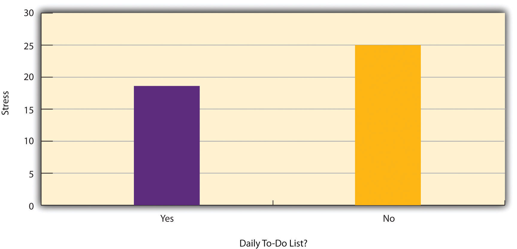
Figure 6.2 shows data from a hypothetical study on the relationship between whether people make a daily list of things to do (a “to-do list”) and stress. Notice that it is unclear whether this is an experiment or a correlational study because it is unclear whether the independent variable was manipulated. If the researcher randomly assigned some participants to make daily to-do lists and others not to, then it is an experiment. If the researcher simply asked participants whether they made daily to-do lists, then it is a correlational study. The distinction is important because if the study was an experiment, then it could be concluded that making the daily to-do lists reduced participants’ stress. But if it was a correlational study, it could only be concluded that these variables are statistically related. Perhaps being stressed has a negative effect on people’s ability to plan ahead (the directionality problem). Or perhaps people who are more conscientious are more likely to make to-do lists and less likely to be stressed (the third-variable problem). The crucial point is that what defines a study as experimental or correlational is not the variables being studied, nor whether the variables are quantitative or categorical, nor the type of graph or statistics used to analyze the data. What defines a study is how the study is conducted.

Data Collection in Correlational Research

Again, the defining feature of correlational research is that neither variable is manipulated. It does not matter how or where the variables are measured. A researcher could have participants come to a laboratory to complete a computerized backward digit span task and a computerized risky decision-making task and then assess the relationship between participants’ scores on the two tasks. Or a researcher could go to a shopping mall to ask people about their attitudes toward the environment and their shopping habits and then assess the relationship between these two variables. Both of these studies would be correlational because no independent variable is manipulated. 

Correlations Between Quantitative Variables

Correlations between quantitative variables are often presented using scatterplots . Figure 6.3 shows some hypothetical data on the relationship between the amount of stress people are under and the number of physical symptoms they have. Each point in the scatterplot represents one person’s score on both variables. For example, the circled point in Figure 6.3 represents a person whose stress score was 10 and who had three physical symptoms. Taking all the points into account, one can see that people under more stress tend to have more physical symptoms. This is a good example of a positive relationship , in which higher scores on one variable tend to be associated with higher scores on the other. In other words, they move in the same direction, either both up or both down. A negative relationship is one in which higher scores on one variable tend to be associated with lower scores on the other. In other words, they move in opposite directions. There is a negative relationship between stress and immune system functioning, for example, because higher stress is associated with lower immune system functioning.

The strength of a correlation between quantitative variables is typically measured using a statistic called  Pearson’s Correlation Coefficient (or Pearson's  r ) . As Figure 6.4 shows, Pearson’s r ranges from −1.00 (the strongest possible negative relationship) to +1.00 (the strongest possible positive relationship). A value of 0 means there is no relationship between the two variables. When Pearson’s  r  is 0, the points on a scatterplot form a shapeless “cloud.” As its value moves toward −1.00 or +1.00, the points come closer and closer to falling on a single straight line. Correlation coefficients near ±.10 are considered small, values near ± .30 are considered medium, and values near ±.50 are considered large. Notice that the sign of Pearson’s  r  is unrelated to its strength. Pearson’s  r  values of +.30 and −.30, for example, are equally strong; it is just that one represents a moderate positive relationship and the other a moderate negative relationship. With the exception of reliability coefficients, most correlations that we find in Psychology are small or moderate in size. The website http://rpsychologist.com/d3/correlation/ , created by Kristoffer Magnusson, provides an excellent interactive visualization of correlations that permits you to adjust the strength and direction of a correlation while witnessing the corresponding changes to the scatterplot.

There are two common situations in which the value of Pearson’s  r  can be misleading. Pearson’s  r  is a good measure only for linear relationships, in which the points are best approximated by a straight line. It is not a good measure for nonlinear relationships, in which the points are better approximated by a curved line. Figure 6.5, for example, shows a hypothetical relationship between the amount of sleep people get per night and their level of depression. In this example, the line that best approximates the points is a curve—a kind of upside-down “U”—because people who get about eight hours of sleep tend to be the least depressed. Those who get too little sleep and those who get too much sleep tend to be more depressed. Even though Figure 6.5 shows a fairly strong relationship between depression and sleep, Pearson’s  r  would be close to zero because the points in the scatterplot are not well fit by a single straight line. This means that it is important to make a scatterplot and confirm that a relationship is approximately linear before using Pearson’s  r . Nonlinear relationships are fairly common in psychology, but measuring their strength is beyond the scope of this book.

The other common situations in which the value of Pearson’s  r  can be misleading is when one or both of the variables have a limited range in the sample relative to the population. This problem is referred to as  restriction of range . Assume, for example, that there is a strong negative correlation between people’s age and their enjoyment of hip hop music as shown by the scatterplot in Figure 6.6. Pearson’s  r  here is −.77. However, if we were to collect data only from 18- to 24-year-olds—represented by the shaded area of Figure 6.6—then the relationship would seem to be quite weak. In fact, Pearson’s  r  for this restricted range of ages is 0. It is a good idea, therefore, to design studies to avoid restriction of range. For example, if age is one of your primary variables, then you can plan to collect data from people of a wide range of ages. Because restriction of range is not always anticipated or easily avoidable, however, it is good practice to examine your data for possible restriction of range and to interpret Pearson’s  r  in light of it. (There are also statistical methods to correct Pearson’s  r  for restriction of range, but they are beyond the scope of this book).

Correlation Does Not Imply Causation

You have probably heard repeatedly that “Correlation does not imply causation.” An amusing example of this comes from a 2012 study that showed a positive correlation (Pearson’s r = 0.79) between the per capita chocolate consumption of a nation and the number of Nobel prizes awarded to citizens of that nation [2] . It seems clear, however, that this does not mean that eating chocolate causes people to win Nobel prizes, and it would not make sense to try to increase the number of Nobel prizes won by recommending that parents feed their children more chocolate.

There are two reasons that correlation does not imply causation. The first is called the  directionality problem . Two variables,  X  and  Y , can be statistically related because X  causes  Y  or because  Y  causes  X . Consider, for example, a study showing that whether or not people exercise is statistically related to how happy they are—such that people who exercise are happier on average than people who do not. This statistical relationship is consistent with the idea that exercising causes happiness, but it is also consistent with the idea that happiness causes exercise. Perhaps being happy gives people more energy or leads them to seek opportunities to socialize with others by going to the gym. The second reason that correlation does not imply causation is called the  third-variable problem . Two variables,  X  and  Y , can be statistically related not because  X  causes  Y , or because  Y  causes  X , but because some third variable,  Z , causes both  X  and  Y . For example, the fact that nations that have won more Nobel prizes tend to have higher chocolate consumption probably reflects geography in that European countries tend to have higher rates of per capita chocolate consumption and invest more in education and technology (once again, per capita) than many other countries in the world. Similarly, the statistical relationship between exercise and happiness could mean that some third variable, such as physical health, causes both of the others. Being physically healthy could cause people to exercise and cause them to be happier. Correlations that are a result of a third-variable are often referred to as  spurious correlations.

Some excellent and amusing examples of spurious correlations can be found at http://www.tylervigen.com  (Figure 6.7  provides one such example).

“Lots of Candy Could Lead to Violence”

Although researchers in psychology know that correlation does not imply causation, many journalists do not. One website about correlation and causation, http://jonathan.mueller.faculty.noctrl.edu/100/correlation_or_causation.htm , links to dozens of media reports about real biomedical and psychological research. Many of the headlines suggest that a causal relationship has been demonstrated when a careful reading of the articles shows that it has not because of the directionality and third-variable problems.

One such article is about a study showing that children who ate candy every day were more likely than other children to be arrested for a violent offense later in life. But could candy really “lead to” violence, as the headline suggests? What alternative explanations can you think of for this statistical relationship? How could the headline be rewritten so that it is not misleading?

As you have learned by reading this book, there are various ways that researchers address the directionality and third-variable problems. The most effective is to conduct an experiment. For example, instead of simply measuring how much people exercise, a researcher could bring people into a laboratory and randomly assign half of them to run on a treadmill for 15 minutes and the rest to sit on a couch for 15 minutes. Although this seems like a minor change to the research design, it is extremely important. Now if the exercisers end up in more positive moods than those who did not exercise, it cannot be because their moods affected how much they exercised (because it was the researcher who used random assignment to determine how much they exercised). Likewise, it cannot be because some third variable (e.g., physical health) affected both how much they exercised and what mood they were in. Thus experiments eliminate the directionality and third-variable problems and allow researchers to draw firm conclusions about causal relationships.

• Explain the purpose of null hypothesis testing, including the role of sampling error.
• Describe the basic logic of null hypothesis testing.
• Describe the role of relationship strength and sample size in determining statistical significance and make reasonable judgments about statistical significance based on these two factors.

 The Purpose of Null Hypothesis Testing

As we have seen, psychological research typically involves measuring one or more variables in a sample and computing descriptive summary data (e.g., means, correlation coefficients) for those variables. These descriptive data for the sample are called statistics .  In general, however, the researcher’s goal is not to draw conclusions about that sample but to draw conclusions about the population that the sample was selected from. Thus researchers must use sample statistics to draw conclusions about the corresponding values in the population. These corresponding values in the population are called parameters . Imagine, for example, that a researcher measures the number of depressive symptoms exhibited by each of 50 adults with clinical depression and computes the mean number of symptoms. The researcher probably wants to use this sample statistic (the mean number of symptoms for the sample) to draw conclusions about the corresponding population parameter (the mean number of symptoms for adults with clinical depression).

Unfortunately, sample statistics are not perfect estimates of their corresponding population parameters. This is because there is a certain amount of random variability in any statistic from sample to sample. The mean number of depressive symptoms might be 8.73 in one sample of adults with clinical depression, 6.45 in a second sample, and 9.44 in a third—even though these samples are selected randomly from the same population. Similarly, the correlation (Pearson’s  r ) between two variables might be +.24 in one sample, −.04 in a second sample, and +.15 in a third—again, even though these samples are selected randomly from the same population. This random variability in a statistic from sample to sample is called  sampling error . (Note that the term error  here refers to random variability and does not imply that anyone has made a mistake. No one “commits a sampling error.”)

One implication of this is that when there is a statistical relationship in a sample, it is not always clear that there is a statistical relationship in the population. A small difference between two group means in a sample might indicate that there is a small difference between the two group means in the population. But it could also be that there is no difference between the means in the population and that the difference in the sample is just a matter of sampling error. Similarly, a Pearson’s  r  value of −.29 in a sample might mean that there is a negative relationship in the population. But it could also be that there is no relationship in the population and that the relationship in the sample is just a matter of sampling error.

In fact, any statistical relationship in a sample can be interpreted in two ways:

• There is a relationship in the population, and the relationship in the sample reflects this.
• There is no relationship in the population, and the relationship in the sample reflects only sampling error.

The purpose of null hypothesis testing is simply to help researchers decide between these two interpretations.

The Logic of Null Hypothesis Testing

Null hypothesis testing (often called null hypothesis significance testing or NHST) is a formal approach to deciding between two interpretations of a statistical relationship in a sample. One interpretation is called the   null hypothesis  (often symbolized  H 0 and read as “H-zero”). This is the idea that there is no relationship in the population and that the relationship in the sample reflects only sampling error. Informally, the null hypothesis is that the sample relationship “occurred by chance.” The other interpretation is called the alternative hypothesis  (often symbolized as  H 1 ). This is the idea that there is a relationship in the population and that the relationship in the sample reflects this relationship in the population.

Again, every statistical relationship in a sample can be interpreted in either of these two ways: It might have occurred by chance, or it might reflect a relationship in the population. So researchers need a way to decide between them. Although there are many specific null hypothesis testing techniques, they are all based on the same general logic. The steps are as follows:

• Assume for the moment that the null hypothesis is true. There is no relationship between the variables in the population.
• Determine how likely the sample relationship would be if the null hypothesis were true.
• If the sample relationship would be extremely unlikely, then reject the null hypothesis  in favor of the alternative hypothesis. If it would not be extremely unlikely, then  retain the null hypothesis .

Following this logic, we can begin to understand why Mehl and his colleagues concluded that there is no difference in talkativeness between women and men in the population. In essence, they asked the following question: “If there were no difference in the population, how likely is it that we would find a small difference of  d  = 0.06 in our sample?” Their answer to this question was that this sample relationship would be fairly likely if the null hypothesis were true. Therefore, they retained the null hypothesis—concluding that there is no evidence of a sex difference in the population. We can also see why Kanner and his colleagues concluded that there is a correlation between hassles and symptoms in the population. They asked, “If the null hypothesis were true, how likely is it that we would find a strong correlation of +.60 in our sample?” Their answer to this question was that this sample relationship would be fairly unlikely if the null hypothesis were true. Therefore, they rejected the null hypothesis in favor of the alternative hypothesis—concluding that there is a positive correlation between these variables in the population.

A crucial step in null hypothesis testing is finding the probability of the sample result or a more extreme result if the null hypothesis were true (Lakens, 2017). [3] This probability is called the p value . A low  p value means that the sample or more extreme result would be unlikely if the null hypothesis were true and leads to the rejection of the null hypothesis. A p value that is not low means that the sample or more extreme result would be likely if the null hypothesis were true and leads to the retention of the null hypothesis. But how low must the p value criterion be before the sample result is considered unlikely enough to reject the null hypothesis? In null hypothesis testing, this criterion is called α (alpha) and is almost always set to .05. If there is a 5% chance or less of a result at least as extreme as the sample result if the null hypothesis were true, then the null hypothesis is rejected. When this happens, the result is said to be statistically significant . If there is greater than a 5% chance of a result as extreme as the sample result when the null hypothesis is true, then the null hypothesis is retained. This does not necessarily mean that the researcher accepts the null hypothesis as true—only that there is not currently enough evidence to reject it. Researchers often use the expression “fail to reject the null hypothesis” rather than “retain the null hypothesis,” but they never use the expression “accept the null hypothesis.”

The Misunderstood  p  Value

The  p  value is one of the most misunderstood quantities in psychological research (Cohen, 1994) [4] . Even professional researchers misinterpret it, and it is not unusual for such misinterpretations to appear in statistics textbooks!

The most common misinterpretation is that the  p  value is the probability that the null hypothesis is true—that the sample result occurred by chance. For example, a misguided researcher might say that because the  p  value is .02, there is only a 2% chance that the result is due to chance and a 98% chance that it reflects a real relationship in the population. But this is incorrect . The  p  value is really the probability of a result at least as extreme as the sample result  if  the null hypothesis  were  true. So a  p  value of .02 means that if the null hypothesis were true, a sample result this extreme would occur only 2% of the time.

You can avoid this misunderstanding by remembering that the  p  value is not the probability that any particular  hypothesis  is true or false. Instead, it is the probability of obtaining the  sample result  if the null hypothesis were true.

Role of Sample Size and Relationship Strength

Recall that null hypothesis testing involves answering the question, “If the null hypothesis were true, what is the probability of a sample result as extreme as this one?” In other words, “What is the  p  value?” It can be helpful to see that the answer to this question depends on just two considerations: the strength of the relationship and the size of the sample. Specifically, the stronger the sample relationship and the larger the sample, the less likely the result would be if the null hypothesis were true. That is, the lower the  p  value. This should make sense. Imagine a study in which a sample of 500 women is compared with a sample of 500 men in terms of some psychological characteristic, and Cohen’s  d  is a strong 0.50. If there were really no sex difference in the population, then a result this strong based on such a large sample should seem highly unlikely. Now imagine a similar study in which a sample of three women is compared with a sample of three men, and Cohen’s  d  is a weak 0.10. If there were no sex difference in the population, then a relationship this weak based on such a small sample should seem likely. And this is precisely why the null hypothesis would be rejected in the first example and retained in the second.

Of course, sometimes the result can be weak and the sample large, or the result can be strong and the sample small. In these cases, the two considerations trade off against each other so that a weak result can be statistically significant if the sample is large enough and a strong relationship can be statistically significant even if the sample is small. Table 13.1 shows roughly how relationship strength and sample size combine to determine whether a sample result is statistically significant. The columns of the table represent the three levels of relationship strength: weak, medium, and strong. The rows represent four sample sizes that can be considered small, medium, large, and extra large in the context of psychological research. Thus each cell in the table represents a combination of relationship strength and sample size. If a cell contains the word  Yes , then this combination would be statistically significant for both Cohen’s  d  and Pearson’s  r . If it contains the word  No , then it would not be statistically significant for either. There is one cell where the decision for  d  and  r  would be different and another where it might be different depending on some additional considerations, which are discussed in Section 13.2 "Some Basic Null Hypothesis Tests"

Although Table 13.1 provides only a rough guideline, it shows very clearly that weak relationships based on medium or small samples are never statistically significant and that strong relationships based on medium or larger samples are always statistically significant. If you keep this lesson in mind, you will often know whether a result is statistically significant based on the descriptive statistics alone. It is extremely useful to be able to develop this kind of intuitive judgment. One reason is that it allows you to develop expectations about how your formal null hypothesis tests are going to come out, which in turn allows you to detect problems in your analyses. For example, if your sample relationship is strong and your sample is medium, then you would expect to reject the null hypothesis. If for some reason your formal null hypothesis test indicates otherwise, then you need to double-check your computations and interpretations. A second reason is that the ability to make this kind of intuitive judgment is an indication that you understand the basic logic of this approach in addition to being able to do the computations.

Statistical Significance Versus Practical Significance

Table 13.1 illustrates another extremely important point. A statistically significant result is not necessarily a strong one. Even a very weak result can be statistically significant if it is based on a large enough sample. This is closely related to Janet Shibley Hyde’s argument about sex differences (Hyde, 2007) [5] . The differences between women and men in mathematical problem solving and leadership ability are statistically significant. But the word  significant  can cause people to interpret these differences as strong and important—perhaps even important enough to influence the college courses they take or even who they vote for. As we have seen, however, these statistically significant differences are actually quite weak—perhaps even “trivial.”

This is why it is important to distinguish between the  statistical  significance of a result and the  practical  significance of that result.  Practical significance refers to the importance or usefulness of the result in some real-world context. Many sex differences are statistically significant—and may even be interesting for purely scientific reasons—but they are not practically significant. In clinical practice, this same concept is often referred to as “clinical significance.” For example, a study on a new treatment for social phobia might show that it produces a statistically significant positive effect. Yet this effect still might not be strong enough to justify the time, effort, and other costs of putting it into practice—especially if easier and cheaper treatments that work almost as well already exist. Although statistically significant, this result would be said to lack practical or clinical significance.

• List the various types of observational research methods and distinguish between each.
• Describe the strengths and weakness of each observational research method. 

What Is Observational Research?

The term observational research is used to refer to several different types of non-experimental studies in which behavior is systematically observed and recorded. The goal of observational research is to describe a variable or set of variables. More generally, the goal is to obtain a snapshot of specific characteristics of an individual, group, or setting. As described previously, observational research is non-experimental because nothing is manipulated or controlled, and as such we cannot arrive at causal conclusions using this approach. The data that are collected in observational research studies are often qualitative in nature but they may also be quantitative or both (mixed-methods). There are several different types of observational methods that will be described below.

Naturalistic Observation

Naturalistic observation  is an observational method that involves observing people’s behavior in the environment in which it typically occurs. Thus naturalistic observation is a type of field research (as opposed to a type of laboratory research). Jane Goodall's famous research on chimpanzees is a classic example of naturalistic observation. Dr.  Goodall spent three decades observing chimpanzees in their natural environment in East Africa. She examined such things as chimpanzee’s social structure, mating patterns, gender roles, family structure, and care of offspring by observing them in the wild. However, naturalistic observation  could more simply involve observing shoppers in a grocery store, children on a school playground, or psychiatric inpatients in their wards. Researchers engaged in naturalistic observation usually make their observations as unobtrusively as possible so that participants are not aware that they are being studied. Such an approach is called disguised naturalistic observation .  Ethically, this method is considered to be acceptable if the participants remain anonymous and the behavior occurs in a public setting where people would not normally have an expectation of privacy. Grocery shoppers putting items into their shopping carts, for example, are engaged in public behavior that is easily observable by store employees and other shoppers. For this reason, most researchers would consider it ethically acceptable to observe them for a study. On the other hand, one of the arguments against the ethicality of the naturalistic observation of “bathroom behavior” discussed earlier in the book is that people have a reasonable expectation of privacy even in a public restroom and that this expectation was violated. 

In cases where it is not ethical or practical to conduct disguised naturalistic observation, researchers can conduct  undisguised naturalistic observation where the participants are made aware of the researcher presence and monitoring of their behavior. However, one concern with undisguised naturalistic observation is  reactivity. Reactivity refers to when a measure changes participants’ behavior. In the case of undisguised naturalistic observation, the concern with reactivity is that when people know they are being observed and studied, they may act differently than they normally would. This type of reactivity is known as the Hawthorne effect . For instance, you may act much differently in a bar if you know that someone is observing you and recording your behaviors and this would invalidate the study. So disguised observation is less reactive and therefore can have higher validity because people are not aware that their behaviors are being observed and recorded. However, we now know that people often become used to being observed and with time they begin to behave naturally in the researcher’s presence. In other words, over time people habituate to being observed. Think about reality shows like Big Brother or Survivor where people are constantly being observed and recorded. While they may be on their best behavior at first, in a fairly short amount of time they are flirting, having sex, wearing next to nothing, screaming at each other, and occasionally behaving in ways that are embarrassing.

Participant Observation

Another approach to data collection in observational research is participant observation. In  participant observation , researchers become active participants in the group or situation they are studying. Participant observation is very similar to naturalistic observation in that it involves observing people’s behavior in the environment in which it typically occurs. As with naturalistic observation, the data that are collected can include interviews (usually unstructured), notes based on their observations and interactions, documents, photographs, and other artifacts. The only difference between naturalistic observation and participant observation is that researchers engaged in participant observation become active members of the group or situations they are studying. The basic rationale for participant observation is that there may be important information that is only accessible to, or can be interpreted only by, someone who is an active participant in the group or situation. Like naturalistic observation, participant observation can be either disguised or undisguised. In disguised participant observation , the researchers pretend to be members of the social group they are observing and conceal their true identity as researchers.

In a famous example of disguised participant observation, Leon Festinger and his colleagues infiltrated a doomsday cult known as the Seekers, whose members believed that the apocalypse would occur on December 21, 1954. Interested in studying how members of the group would cope psychologically when the prophecy inevitably failed, they carefully recorded the events and reactions of the cult members in the days before and after the supposed end of the world. Unsurprisingly, the cult members did not give up their belief but instead convinced themselves that it was their faith and efforts that saved the world from destruction. Festinger and his colleagues later published a book about this experience, which they used to illustrate the theory of cognitive dissonance (Festinger, Riecken, & Schachter, 1956) [6] .

In contrast with undisguised participant observation ,  the researchers become a part of the group they are studying and they disclose their true identity as researchers to the group under investigation. Once again there are important ethical issues to consider with disguised participant observation.  First no informed consent can be obtained and second deception is being used. The researcher is deceiving the participants by intentionally withholding information about their motivations for being a part of the social group they are studying. But sometimes disguised participation is the only way to access a protective group (like a cult). Further, disguised participant observation is less prone to reactivity than undisguised participant observation. 

Rosenhan’s study (1973) [7]   of the experience of people in a psychiatric ward would be considered disguised participant observation because Rosenhan and his pseudopatients were admitted into psychiatric hospitals on the pretense of being patients so that they could observe the way that psychiatric patients are treated by staff. The staff and other patients were unaware of their true identities as researchers.

Another example of participant observation comes from a study by sociologist Amy Wilkins on a university-based religious organization that emphasized how happy its members were (Wilkins, 2008) [8] . Wilkins spent 12 months attending and participating in the group’s meetings and social events, and she interviewed several group members. In her study, Wilkins identified several ways in which the group “enforced” happiness—for example, by continually talking about happiness, discouraging the expression of negative emotions, and using happiness as a way to distinguish themselves from other groups.

One of the primary benefits of participant observation is that the researchers are in a much better position to understand the viewpoint and experiences of the people they are studying when they are a part of the social group. The primary limitation with this approach is that the mere presence of the observer could affect the behavior of the people being observed. While this is also a concern with naturalistic observation, additional concerns arise when researchers become active members of the social group they are studying because that they may change the social dynamics and/or influence the behavior of the people they are studying. Similarly, if the researcher acts as a participant observer there can be concerns with biases resulting from developing relationships with the participants. Concretely, the researcher may become less objective resulting in more experimenter bias.

Structured Observation

Another observational method is structured observation . Here the investigator makes careful observations of one or more specific behaviors in a particular setting that is more structured than the settings used in naturalistic or participant observation. Often the setting in which the observations are made is not the natural setting. Instead, the researcher may observe people in the laboratory environment. Alternatively, the researcher may observe people in a natural setting (like a classroom setting) that they have structured some way, for instance by introducing some specific task participants are to engage in or by introducing a specific social situation or manipulation.

Structured observation is very similar to naturalistic observation and participant observation in that in all three cases researchers are observing naturally occurring behavior; however, the emphasis in structured observation is on gathering quantitative rather than qualitative data. Researchers using this approach are interested in a limited set of behaviors. This allows them to quantify the behaviors they are observing. In other words, structured observation is less global than naturalistic or participant observation because the researcher engaged in structured observations is interested in a small number of specific behaviors. Therefore, rather than recording everything that happens, the researcher only focuses on very specific behaviors of interest.

Researchers Robert Levine and Ara Norenzayan used structured observation to study differences in the “pace of life” across countries (Levine & Norenzayan, 1999) [9] . One of their measures involved observing pedestrians in a large city to see how long it took them to walk 60 feet. They found that people in some countries walked reliably faster than people in other countries. For example, people in Canada and Sweden covered 60 feet in just under 13 seconds on average, while people in Brazil and Romania took close to 17 seconds. When structured observation  takes place in the complex and even chaotic “real world,” the questions of when, where, and under what conditions the observations will be made, and who exactly will be observed are important to consider. Levine and Norenzayan described their sampling process as follows:

“Male and female walking speed over a distance of 60 feet was measured in at least two locations in main downtown areas in each city. Measurements were taken during main business hours on clear summer days. All locations were flat, unobstructed, had broad sidewalks, and were sufficiently uncrowded to allow pedestrians to move at potentially maximum speeds. To control for the effects of socializing, only pedestrians walking alone were used. Children, individuals with obvious physical handicaps, and window-shoppers were not timed. Thirty-five men and 35 women were timed in most cities.” (p. 186).

Precise specification of the sampling process in this way makes data collection manageable for the observers, and it also provides some control over important extraneous variables. For example, by making their observations on clear summer days in all countries, Levine and Norenzayan controlled for effects of the weather on people’s walking speeds.  In Levine and Norenzayan’s study, measurement was relatively straightforward. They simply measured out a 60-foot distance along a city sidewalk and then used a stopwatch to time participants as they walked over that distance.

As another example, researchers Robert Kraut and Robert Johnston wanted to study bowlers’ reactions to their shots, both when they were facing the pins and then when they turned toward their companions (Kraut & Johnston, 1979) [10] . But what “reactions” should they observe? Based on previous research and their own pilot testing, Kraut and Johnston created a list of reactions that included “closed smile,” “open smile,” “laugh,” “neutral face,” “look down,” “look away,” and “face cover” (covering one’s face with one’s hands). The observers committed this list to memory and then practiced by coding the reactions of bowlers who had been videotaped. During the actual study, the observers spoke into an audio recorder, describing the reactions they observed. Among the most interesting results of this study was that bowlers rarely smiled while they still faced the pins. They were much more likely to smile after they turned toward their companions, suggesting that smiling is not purely an expression of happiness but also a form of social communication.

In yet another example (this one in a laboratory environment), Dov Cohen and his colleagues had observers rate the emotional reactions of participants who had just been deliberately bumped and insulted by a confederate after they dropped off a completed questionnaire at the end of a hallway. The confederate was posing as someone who worked in the same building and who was frustrated by having to close a file drawer twice in order to permit the participants to walk past them (first to drop off the questionnaire at the end of the hallway and once again on their way back to the room where they believed the study they signed up for was taking place). The two observers were positioned at different ends of the hallway so that they could read the participants' body language and hear anything they might say. Interestingly, the researchers hypothesized that participants from the southern United States, which is one of several places in the world that has a "culture of honor," would react with more aggression than participants from the northern United States, a prediction that was in fact supported by the observational data (Cohen, Nisbett, Bowdle, & Schwarz, 1996) [11] .

When the observations require a judgment on the part of the observers—as in the studies by Kraut and Johnston and Cohen and his colleagues—a process referred to as   coding is typically required . Coding generally requires clearly defining a set of target behaviors. The observers then categorize participants individually in terms of which behavior they have engaged in and the number of times they engaged in each behavior. The observers might even record the duration of each behavior. The target behaviors must be defined in such a way that guides different observers to code them in the same way. This difficulty with coding illustrates the issue of interrater reliability, as mentioned in Chapter 4. Researchers are expected to demonstrate the interrater reliability of their coding procedure by having multiple raters code the same behaviors independently and then showing that the different observers are in close agreement. Kraut and Johnston, for example, video recorded a subset of their participants’ reactions and had two observers independently code them. The two observers showed that they agreed on the reactions that were exhibited 97% of the time, indicating good interrater reliability.

One of the primary benefits of structured observation is that it is far more efficient than naturalistic and participant observation. Since the researchers are focused on specific behaviors this reduces time and expense. Also, often times the environment is structured to encourage the behaviors of interest which again means that researchers do not have to invest as much time in waiting for the behaviors of interest to naturally occur. Finally, researchers using this approach can clearly exert greater control over the environment. However, when researchers exert more control over the environment it may make the environment less natural which decreases external validity. It is less clear for instance whether structured observations made in a laboratory environment will generalize to a real world environment. Furthermore, since researchers engaged in structured observation are often not disguised there may be more concerns with reactivity.

Case Studies

A  case study   is an in-depth examination of an individual. Sometimes case studies are also completed on social units (e.g., a cult) and events (e.g., a natural disaster). Most commonly in psychology, however, case studies provide a detailed description and analysis of an individual. Often the individual has a rare or unusual condition or disorder or has damage to a specific region of the brain.

Like many observational research methods, case studies tend to be more qualitative in nature. Case study methods involve an in-depth, and often a longitudinal examination of an individual. Depending on the focus of the case study, individuals may or may not be observed in their natural setting. If the natural setting is not what is of interest, then the individual may be brought into a therapist’s office or a researcher’s lab for study. Also, the bulk of the case study report will focus on in-depth descriptions of the person rather than on statistical analyses. With that said some quantitative data may also be included in the write-up of a case study. For instance, an individual's depression score may be compared to normative scores or their score before and after treatment may be compared. As with other qualitative methods, a variety of different methods and tools can be used to collect information on the case. For instance, interviews, naturalistic observation, structured observation, psychological testing (e.g., IQ test), and/or physiological measurements (e.g., brain scans) may be used to collect information on the individual.

HM is one of the most notorious case studies in psychology. HM suffered from intractable and very severe epilepsy. A surgeon localized HM’s epilepsy to his medial temporal lobe and in 1953 he removed large sections of his hippocampus in an attempt to stop the seizures. The treatment was a success, in that it resolved his epilepsy and his IQ and personality were unaffected. However, the doctors soon realized that HM exhibited a strange form of amnesia, called anterograde amnesia. HM was able to carry out a conversation and he could remember short strings of letters, digits, and words. Basically, his short term memory was preserved. However, HM could not commit new events to memory. He lost the ability to transfer information from his short-term memory to his long term memory, something memory researchers call consolidation. So while he could carry on a conversation with someone, he would completely forget the conversation after it ended. This was an extremely important case study for memory researchers because it suggested that there’s a dissociation between short-term memory and long-term memory, it suggested that these were two different abilities sub-served by different areas of the brain. It also suggested that the temporal lobes are particularly important for consolidating new information (i.e., for transferring information from short-term memory to long-term memory).

The history of psychology is filled with influential cases studies, such as Sigmund Freud’s description of “Anna O.” (see Note 6.1 "The Case of “Anna O.”") and John Watson and Rosalie Rayner’s description of Little Albert (Watson & Rayner, 1920) [12] , who allegedly learned to fear a white rat—along with other furry objects—when the researchers repeatedly made a loud noise every time the rat approached him.

The Case of “Anna O.”

Sigmund Freud used the case of a young woman he called “Anna O.” to illustrate many principles of his theory of psychoanalysis (Freud, 1961) [13] . (Her real name was Bertha Pappenheim, and she was an early feminist who went on to make important contributions to the field of social work.) Anna had come to Freud’s colleague Josef Breuer around 1880 with a variety of odd physical and psychological symptoms. One of them was that for several weeks she was unable to drink any fluids. According to Freud,

She would take up the glass of water that she longed for, but as soon as it touched her lips she would push it away like someone suffering from hydrophobia.…She lived only on fruit, such as melons, etc., so as to lessen her tormenting thirst. (p. 9)

But according to Freud, a breakthrough came one day while Anna was under hypnosis.

[S]he grumbled about her English “lady-companion,” whom she did not care for, and went on to describe, with every sign of disgust, how she had once gone into this lady’s room and how her little dog—horrid creature!—had drunk out of a glass there. The patient had said nothing, as she had wanted to be polite. After giving further energetic expression to the anger she had held back, she asked for something to drink, drank a large quantity of water without any difficulty, and awoke from her hypnosis with the glass at her lips; and thereupon the disturbance vanished, never to return. (p.9)

Freud’s interpretation was that Anna had repressed the memory of this incident along with the emotion that it triggered and that this was what had caused her inability to drink. Furthermore, he believed that her recollection of the incident, along with her expression of the emotion she had repressed, caused the symptom to go away.

As an illustration of Freud’s theory, the case study of Anna O. is quite effective. As evidence for the theory, however, it is essentially worthless. The description provides no way of knowing whether Anna had really repressed the memory of the dog drinking from the glass, whether this repression had caused her inability to drink, or whether recalling this “trauma” relieved the symptom. It is also unclear from this case study how typical or atypical Anna’s experience was.

Case studies are useful because they provide a level of detailed analysis not found in many other research methods and greater insights may be gained from this more detailed analysis. As a result of the case study, the researcher may gain a sharpened understanding of what might become important to look at more extensively in future more controlled research. Case studies are also often the only way to study rare conditions because it may be impossible to find a large enough sample of individuals with the condition to use quantitative methods. Although at first glance a case study of a rare individual might seem to tell us little about ourselves, they often do provide insights into normal behavior. The case of HM provided important insights into the role of the hippocampus in memory consolidation.

However, it is important to note that while case studies can provide insights into certain areas and variables to study, and can be useful in helping develop theories, they should never be used as evidence for theories. In other words, case studies can be used as inspiration to formulate theories and hypotheses, but those hypotheses and theories then need to be formally tested using more rigorous quantitative methods. The reason case studies shouldn’t be used to provide support for theories is that they suffer from problems with both internal and external validity. Case studies lack the proper controls that true experiments contain. As such, they suffer from problems with internal validity, so they cannot be used to determine causation. For instance, during HM’s surgery, the surgeon may have accidentally lesioned another area of HM's brain (a possibility suggested by the dissection of HM's brain following his death) and that lesion may have contributed to his inability to consolidate new information. The fact is, with case studies we cannot rule out these sorts of alternative explanations. So, as with all observational methods, case studies do not permit determination of causation. In addition, because case studies are often of a single individual, and typically an abnormal individual, researchers cannot generalize their conclusions to other individuals. Recall that with most research designs there is a trade-off between internal and external validity. With case studies, however, there are problems with both internal validity and external validity. So there are limits both to the ability to determine causation and to generalize the results. A final limitation of case studies is that ample opportunity exists for the theoretical biases of the researcher to color or bias the case description. Indeed, there have been accusations that the woman who studied HM destroyed a lot of her data that were not published and she has been called into question for destroying contradictory data that didn’t support her theory about how memories are consolidated. There is a fascinating New York Times article that describes some of the controversies that ensued after HM's death and analysis of his brain that can be found at: https://www.nytimes.com/2016/08/07/magazine/the-brain-that-couldnt-remember.html?_r=0

Archival Research

Another approach that is often considered observational research involves analyzing archival data that have already been collected for some other purpose. An example is a study by Brett Pelham and his colleagues on “implicit egotism”—the tendency for people to prefer people, places, and things that are similar to themselves (Pelham, Carvallo, & Jones, 2005) [14] . In one study, they examined Social Security records to show that women with the names Virginia, Georgia, Louise, and Florence were especially likely to have moved to the states of Virginia, Georgia, Louisiana, and Florida, respectively.

As with naturalistic observation, measurement can be more or less straightforward when working with archival data. For example, counting the number of people named Virginia who live in various states based on Social Security records is relatively straightforward. But consider a study by Christopher Peterson and his colleagues on the relationship between optimism and health using data that had been collected many years before for a study on adult development (Peterson, Seligman, & Vaillant, 1988) [15] . In the 1940s, healthy male college students had completed an open-ended questionnaire about difficult wartime experiences. In the late 1980s, Peterson and his colleagues reviewed the men’s questionnaire responses to obtain a measure of explanatory style—their habitual ways of explaining bad events that happen to them. More pessimistic people tend to blame themselves and expect long-term negative consequences that affect many aspects of their lives, while more optimistic people tend to blame outside forces and expect limited negative consequences. To obtain a measure of explanatory style for each participant, the researchers used a procedure in which all negative events mentioned in the questionnaire responses, and any causal explanations for them were identified and written on index cards. These were given to a separate group of raters who rated each explanation in terms of three separate dimensions of optimism-pessimism. These ratings were then averaged to produce an explanatory style score for each participant. The researchers then assessed the statistical relationship between the men’s explanatory style as undergraduate students and archival measures of their health at approximately 60 years of age. The primary result was that the more optimistic the men were as undergraduate students, the healthier they were as older men. Pearson’s  r  was +.25.

This method is an example of  content analysis —a family of systematic approaches to measurement using complex archival data. Just as structured observation requires specifying the behaviors of interest and then noting them as they occur, content analysis requires specifying keywords, phrases, or ideas and then finding all occurrences of them in the data. These occurrences can then be counted, timed (e.g., the amount of time devoted to entertainment topics on the nightly news show), or analyzed in a variety of other ways.

• Explain some reasons that researchers use complex correlational designs.
• Create and interpret a correlation matrix.
• Describe how researchers can use partial correlation and multiple regression to statistically control for third variables.

As we have already seen, researchers conduct correlational studies rather than experiments when they are interested in noncausal relationships or when they are interested in causal relationships but the independent variable cannot be manipulated for practical or ethical reasons. In this section, we look at some approaches to complex correlational research that involve measuring several variables and assessing the relationships among them.

Assessing Relationships Among Multiple Variables

Most complex correlational research involves measuring several variables—either binary or continuous—and then assessing the statistical relationships among them. For example, researchers Nathan Radcliffe and William Klein studied a sample of middle-aged adults to see how their level of optimism (measured by using a short questionnaire called the Life Orientation Test) relates to several other variables related to having a heart attack (Radcliffe & Klein, 2002) [16] . These included their health, their knowledge of heart attack risk factors, and their beliefs about their own risk of having a heart attack. They found that more optimistic participants were healthier (e.g., they exercised more and had lower blood pressure), knew about heart attack risk factors, and correctly believed their own risk to be lower than that of their peers.

In another example, Ernest Jouriles and his colleagues measured adolescents' experiences of physical and psychological relationship aggression and their psychological distress. Because measures of physical aggression (such as the Conflict in Adolescent Dating Relationships Inventory and the Relationship Violence Interview) often tend to result in highly skewed distributions, the researchers transformed their measures of physical aggression into a dichotomous (i.e., binary) measure (0 = did not occur, 1 = did occur). They did the same with their measures of psychological aggression and then measured the correlations among these variables, finding that adolescents who experienced physical aggression were moderately likely to also have experienced psychological aggression and that experiencing psychological aggression was related to symptoms of psychological distress. (Jouriles, Garrido, Rosenfield, & McDonald, 2009) [17]

This approach is often used to assess the validity of new psychological measures. For example, when John Cacioppo and Richard Petty created their Need for Cognition Scale—a measure of the extent to which people like to think and value thinking—they used it to measure the need for cognition for a large sample of college students, along with three other variables: intelligence, socially desirable responding (the tendency to give what one thinks is the “appropriate” response), and dogmatism (Caccioppo & Petty, 1982) [18] . The results of this study are summarized in Table 6.1, which is a  correlation matrix  showing the correlation (Pearson’s  r ) between every possible pair of variables in the study. For example, the correlation between the need for cognition and intelligence was +.39, the correlation between intelligence and socially desirable responding was +.02, and so on. (Only half the matrix is filled in because the other half would contain exactly the same information. Also, because the correlation between a variable and itself is always +1.00, these values are replaced with dashes throughout the matrix.) In this case, the overall pattern of correlations was consistent with the researchers’ ideas about how scores on the need for cognition should be related to these other constructs.

Table 6.1 Correlation Matrix Showing Correlations Among the Need for Cognition and Three Other Variables Based on Research by Cacioppo and Petty (1982)

Factor Analysis

When researchers study relationships among a large number of conceptually similar variables, they often use a complex statistical technique called factor analysis . In essence, factor analysis organizes the variables into a smaller number of clusters, such that they are strongly correlated within each cluster but weakly correlated between clusters. Each cluster is then interpreted as multiple measures of the same underlying construct. These underlying constructs are also called “factors.” For example, when people perform a wide variety of mental tasks, factor analysis typically organizes them into two main factors—one that researchers interpret as mathematical intelligence (arithmetic, quantitative estimation, spatial reasoning, and so on) and another that they interpret as verbal intelligence (grammar, reading comprehension, vocabulary, and so on). The Big Five personality factors have been identified through factor analyses of people’s scores on a large number of more specific traits. For example, measures of warmth, gregariousness, activity level, and positive emotions tend to be highly correlated with each other and are interpreted as representing the construct of extraversion. As a final example, researchers Peter Rentfrow and Samuel Gosling asked more than 1,700 university students to rate how much they liked 14 different popular genres of music (Rentfrow & Gosling, 2008) [19] . They then submitted these 14 variables to a factor analysis, which identified four distinct factors. The researchers called them  Reflective and Complex  (blues, jazz, classical, and folk),  Intense and Rebellious  (rock, alternative, and heavy metal),  Upbeat and Conventional  (country, soundtrack, religious, pop), and  Energetic and Rhythmic (rap/hip-hop, soul/funk, and electronica); see Table 6.2.

Table 6.2 Factor Loadings of the 14 Music Genres on Four Varimax-Rotated Principal Components. Based on Research by Rentfrow and Gosling (2003)

Two additional points about factor analysis are worth making here. One is that factors are not categories. Factor analysis does not tell us that people are  either extraverted  or  conscientious or that they like  either  “reflective and complex” music  or  “intense and rebellious” music. Instead, factors are constructs that operate independently of each other. So people who are high in extraversion might be high or low in conscientiousness, and people who like reflective and complex music might or might not also like intense and rebellious music. The second point is that factor analysis reveals only the underlying structure of the variables. It is up to researchers to interpret and label the factors and to explain the origin of that particular factor structure. For example, one reason that extraversion and the other Big Five operate as separate factors is that they appear to be controlled by different genes (Plomin, DeFries, McClean, & McGuffin, 2008) [20] .

Exploring Causal Relationships

Another important use of complex correlational research is to explore possible causal relationships among variables. This might seem surprising given the oft-quoted saying that "correlation does not imply causation.” It is true that correlational research cannot unambiguously establish that one variable causes another. Complex correlational research, however, can often be used to rule out other plausible interpretations. The primary way of doing this is through the statistical control of potential third variables. Instead of controlling these variables through random assignment or by holding them constant as in an experiment, the researcher instead measures them and includes them in the statistical analysis called  partial correlation . Using this technique, researchers can examine the relationship between two variables, while statistically controlling for one or more potential third variables.

For example, assume a researcher was interested in the relationship between watching violent television shows and aggressive behavior but she was concerned that socioeconomic status (SES) might represent a third variable that is driving this relationship. In this case, she could conduct a study in which she measures the amount of violent television that participants watch in their everyday life, the number of acts of aggression that they have engaged in, and their SES. She could first examine the correlation between violent television viewing and aggression. Let's say she found a correlation of +.35, which would be considered a moderate sized positive correlation. Next, she could use partial correlation to reexamine this relationship after statistically controlling for SES. This technique would allow her to examine the relationship between the part of violent television viewing that is independent of SES and the part of aggressive behavior that is independent of SES. If she found that the partial correlation between violent television viewing and aggression while controlling for SES was +.34, that would suggest that the relationship between violent television viewing and aggression is largely independent of SES (i.e., SES is not a third variable driving this relationship). On the other hand, if she found that after statistically controlling for SES the correlation between violent television viewing and aggression dropped to +.03, then that would suggest that SES is indeed a third variable that is driving the relationship. If, however, she found that statistically controlling for SES reduced the magnitude of the correlation from +.35 to +.20, then this would suggest that SES accounts for some, but not all, of the relationship between television violence and aggression. It is important to note that while partial correlation provides an important tool for researchers to statistically control for third variables, researchers using this technique are still limited in their ability to arrive at causal conclusions because this technique does not take care of the directionality problem and there may be other third variables driving the relationship that the researcher did not consider and statistically control.

Once a relationship between two variables has been established, researchers can use that information to make predictions about the value of one variable given the value of another variable. For, instance, once we have established that there is a correlation between IQ and GPA we can use people's IQ scores to predict their GPA. Thus, while correlation coefficients can be used to describe the strength and direction of relationships between variables, regression  is a statistical technique that allows researchers to predict one variable given another. Regression can also be used to describe more complex relationships between more than two variables. Typically the variable that is used to make the prediction is referred to as the  predictor variable  and the variable that is being predicted is called the  outcome variable or criterion variable.  This regression equation has the following general form:

Y = b 1 X 1

 Y in this formula represents the person's predicted score on the outcome variable, b 1   represents the slope of the line depicting the relationship between two variables (or the regression weight), and X 1  represents the person's score on the predictor variable. You can see that to predict a person's score on the outcome variable (Y), one simply needs to multiply their score on the predictor variable (X) by the regression weight ( b 1 )

While simple regression  involves using one variable to predict another,  multiple regression   involves measuring several variables ( X1, X2, X3,…Xi ), and using them to predict some outcome variable ( Y ). Multiple regression can also be used to simply describe the relationship between a single outcome variable (Y) and a set of predictor variables ( X1, X2, X3,…Xi ). The result of a multiple regression analysis is an equation that expresses the outcome variable as an additive combination of the predictor variables. This regression equation has the following general form:

Y = b 1 X 1 + b 2 X 2 + b 3 X 3 + … + b i X i 

The regression weights ( b 1 , b 2 , and so on) indicate how large a contribution a predictor variable makes, on average, to the prediction of the outcome variable. Specifically, they indicate how much the outcome variable changes for each one-unit change in the predictor variable.

The advantage of multiple regression is that it can show whether a predictor variable makes a contribution to an outcome variable  over and above  the contributions made by other predictor variables (i.e., it can be used to show whether a predictor variable is related to an outcome variable after statistically controlling for other predictor variables). As a hypothetical example, imagine that a researcher wants to know how income and health relate to happiness. This is tricky because income and health are themselves related to each other. Thus if people with greater incomes tend to be happier, then perhaps this is only because they tend to be healthier. Likewise, if people who are healthier tend to be happier, perhaps this is only because they tend to make more money. But a multiple regression analysis including both income and health as predictor variables would show whether each one makes a contribution to the prediction of happiness when the other is taken into account (when it is statistically controlled). In other words, multiple regression would allow the researcher to examine whether that part of income that is unrelated to health predicts or relates to happiness as well as whether that part of health that is unrelated to income predicts or relates to happiness. Research like this, by the way, has shown both income and health make extremely small contributions to happiness except in the case of severe poverty or illness (Diener, 2000 [21] ).

The examples discussed in this section only scratch the surface of how researchers use complex correlational research to explore possible causal relationships among variables. It is important to keep in mind, however, that purely correlational approaches cannot unambiguously establish that one variable causes another. The best they can do is show patterns of relationships that are consistent with some causal interpretations and inconsistent with others.

Research Methods in Psychology Copyright © 2020 by Rajiv S. Jhangiani, I-Chant A. Chiang, Carrie Cuttler, Dana C. Leighton & Molly A. Metz is licensed under a Creative Commons Attribution-NonCommercial-ShareAlike 4.0 International License , except where otherwise noted.

Share This Book

Achilleas Kostoulas

Applied Linguistics & Language Teacher Education

Doing research without a control group

I was recently asked by a student whether it is possible to do a research project without a control group, and I am copying my answer here, in case it is of interest to readers of the blog. The TL;DR is that you can , but if you need a more detailed explanation, you can find it in the paragraphs that follow.

In this article you will learn:

• What a control group is;
• Whether a control group is always necessary ;
• Why omitting the control group could be a problem ;
• When you might consider avoiding a control group.

Disclaimer: The primary audience to whom this article is addressed is students doing coursework in applied linguistics , TESOL/ELT and education and similar fields. Chances are that the content applies equally well to other research areas, but it is possible that there are disciplinary differences that you need to be aware of. If you are working in different fields, you will probably need to discuss this matter further with your research supervisor.

What is a control group?

When we do experimental research, it is common practice to divide our sample in two groups. One group (the ‘ intervention ‘ or ‘experimental’ group) is the people on whom we test whatever new idea or method we want to measure. The other group, or control group , usually goes about doing whatever they did, except they get tested in the same ways as the intervention group. This provides us with some ‘baseline’ information about what ‘normal’ outcomes are, which we can then compare with those in the actual intervention group.

You can read more about experimental design, control and intervention groups by following this link .

Is a control group necessary?

Although a two-group design is the simplest and probably most common experimental format, your research questions might suggest a different approach. This was why one of my students came up to me with the following question:

When can I omit or not use the control group in my research, and can I use more than one experimental groups instead? Sometimes we have to do this in Education. When and why?

Such an approach, which uses two experimental groups and no control group is indeed possible, and sometimes appropriate. For example, it is a cost-effective way to measure the effectiveness of two activities, coursebooks or teaching approaches. I will use the term ‘ variables ‘ to describe these things that we are interested in comparing.

Provided that our sample is large enough, and we group membership randomly , we can assume that all the experimental groups are more-or-less similar in most respects, except for the variables that we are comparing. If we then apply a different intervention to each group, we can reasonably assume that it is the different variables that are causing any differences in learning outcomes.

An example of a study with no control group

Suppose we want to improve our students’ fluency in a foreign language. It seems plausible that the more input learners are exposed to, the more fluent they become. However, if we only have budget for either a new library or new audiovisual equipment, we should find out whether it’s more effective for students to spend more time reading or listening.

To find out more, we could assign students to two intervention groups, one of which would spend an hour a week watching TV programming in a foreign language, while the other would spend an hour a week reading books. By measuring the students’ fluency before and after the interventions, we’d be able to make an evidence-based claim about which method is more effective.

Are there problems with omitting a control group?

Without a control group, you cannot be certain that the outcomes are the result of our intervention

Research designs without a control group are useful for answering many simple questions about language teaching and learning, but they come with an important limitation: We cannot be certain that it is our interventions that are producing whatever outcomes we measure.

In the example above, it is possible that students became more fluent because they had more practice speaking at school; or perhaps they became more confident as they grew older; or maybe they just practiced more, because they knew that were being tested (a phenomenon known as the Hawthorne effect ). So, while we might claim that watching television proved more (or less) strongly associated with developing fluency compared to reading, we cannot claim with equal confidence that “if you want to become more fluent you need to watch more television”.

What’s the verdict?

So then, when should we use more than one experimental groups without a control? Ideally, you would use this design only when there is enough evidence in the literature that the intervention you are making is associated with some outcomes, and you are therefore only interested in comparisons. For example, you might know that method A works, and you also know that method B works, so you just want to find out which of the two is more effective. This is something that you will have to establish in the literature review.

If you cannot find enough evidence in the literature to establish this connection, but there are also insurmountable pragmatic reasons why you cannot use a control group (e.g., because you don’t have access to enough participants), then you would have to acknowledge the lack of a control as a limitation of the study when reporting your findings.

If you landed on this page looking for information that will help you with your research project, I hope that the content of this article was of some use. I am happy to answer any other questions you might have, if you’d like to share them as a comment under this post or by contacting me directly. Please feel free to use the social sharing buttons at the bottom of the page to forward this article to anyone who might find this information useful.

Further reading

• Seliger, H. W., & Shohamy, E. (1989). Second Language Research Methods. Oxford: Oxford University Press. pp. 140-141.
• Brown, J. D., & Rodgers, T. S. (2002). Doing Second Language Research. Oxford: Oxford University Press. pp. 211-213
• Dörnyei, Z. (2007). Research Methods in Applied Linguistics: Quantitative, Qualitative, and Mixed Methodologies. Oxford: Oxford University Press. pp. 116-117

About this post: This post was originally published in December 2013, in response to a student query. It was revised, for reader-friendliness, in February 2020.

Share this:

4 responses to “doing research without a control group”.

i found your article helpful. i would like to contact you personally.

This was extremely helpful and i think the only article i could find after 3 pages of google search. THANK YOU!!

That was really very helpful. Thank you very much indeed.

I have an important enquiry. Can I have one control group and two experimental groups even if that would mean including all the population (Yemeni sophomore EFL students at Sana’a University)? Will I face any problems while interpreting the results or generalizing them? Can I, instead, widen the population and make it the “Yemeni EFL students at Sana’a University” and make “Yemeni sophomore EFL students at Sana’a University” as the sample?

It all depends on your research questions, but there seems no reason why you shouldn’t have two experimental groups in addition to your control group. Good luck with your project!

Leave a Reply Cancel reply

This site uses Akismet to reduce spam. Learn how your comment data is processed .

Discover more from Achilleas Kostoulas

Subscribe now to keep reading and get access to the full archive.

Type your email…

Continue reading

Want to create or adapt books like this? Learn more about how Pressbooks supports open publishing practices.

8.2 Quasi-experimental and pre-experimental designs

Learning objectives.

• Identify and describe the various types of quasi-experimental designs
• Distinguish true experimental designs from quasi-experimental and pre-experimental designs
• Identify and describe the various types of quasi-experimental and pre-experimental designs

As we discussed in the previous section, time, funding, and ethics may limit a researcher’s ability to conduct a true experiment. For researchers in the medical sciences and social work, conducting a true experiment could require denying needed treatment to clients, which is a clear ethical violation. Even those whose research may not involve the administration of needed medications or treatments may be limited in their ability to conduct a classic experiment. When true experiments are not possible, researchers often use quasi-experimental designs.

Quasi-experimental designs

Quasi-experimental designs are similar to true experiments, but they lack random assignment to experimental and control groups. Quasi-experimental designs have a comparison group that is similar to a control group except assignment to the comparison group is not determined by random assignment. The most basic of these quasi-experimental designs is the nonequivalent comparison groups design (Rubin & Babbie, 2017).  The nonequivalent comparison group design looks a lot like the classic experimental design, except it does not use random assignment. In many cases, these groups may already exist. For example, a researcher might conduct research at two different agency sites, one of which receives the intervention and the other does not. No one was assigned to treatment or comparison groups. Those groupings existed prior to the study. While this method is more convenient for real-world research, it is less likely that that the groups are comparable than if they had been determined by random assignment. Perhaps the treatment group has a characteristic that is unique–for example, higher income or different diagnoses–that make the treatment more effective.

Quasi-experiments are particularly useful in social welfare policy research. Social welfare policy researchers often look for what are termed natural experiments , or situations in which comparable groups are created by differences that already occur in the real world. Natural experiments are a feature of the social world that allows researchers to use the logic of experimental design to investigate the connection between variables. For example, Stratmann and Wille (2016) were interested in the effects of a state healthcare policy called Certificate of Need on the quality of hospitals. They clearly could not randomly assign states to adopt one set of policies or another. Instead, researchers used hospital referral regions, or the areas from which hospitals draw their patients, that spanned across state lines. Because the hospitals were in the same referral region, researchers could be pretty sure that the client characteristics were pretty similar. In this way, they could classify patients in experimental and comparison groups without dictating state policy or telling people where to live.

Matching is another approach in quasi-experimental design for assigning people to experimental and comparison groups. It begins with researchers thinking about what variables are important in their study, particularly demographic variables or attributes that might impact their dependent variable. Individual matching involves pairing participants with similar attributes. Then, the matched pair is split—with one participant going to the experimental group and the other to the comparison group. An ex post facto control group , in contrast, is when a researcher matches individuals after the intervention is administered to some participants. Finally, researchers may engage in aggregate matching , in which the comparison group is determined to be similar on important variables.

Time series design

There are many different quasi-experimental designs in addition to the nonequivalent comparison group design described earlier. Describing all of them is beyond the scope of this textbook, but one more design is worth mentioning. The time series design uses multiple observations before and after an intervention. In some cases, experimental and comparison groups are used. In other cases where that is not feasible, a single experimental group is used. By using multiple observations before and after the intervention, the researcher can better understand the true value of the dependent variable in each participant before the intervention starts. Additionally, multiple observations afterwards allow the researcher to see whether the intervention had lasting effects on participants. Time series designs are similar to single-subjects designs, which we will discuss in Chapter 15.

Pre-experimental design

When true experiments and quasi-experiments are not possible, researchers may turn to a pre-experimental design (Campbell & Stanley, 1963).  Pre-experimental designs are called such because they often happen as a pre-cursor to conducting a true experiment.  Researchers want to see if their interventions will have some effect on a small group of people before they seek funding and dedicate time to conduct a true experiment. Pre-experimental designs, thus, are usually conducted as a first step towards establishing the evidence for or against an intervention. However, this type of design comes with some unique disadvantages, which we’ll describe below.

A commonly used type of pre-experiment is the one-group pretest post-test design . In this design, pre- and posttests are both administered, but there is no comparison group to which to compare the experimental group. Researchers may be able to make the claim that participants receiving the treatment experienced a change in the dependent variable, but they cannot begin to claim that the change was the result of the treatment without a comparison group.   Imagine if the students in your research class completed a questionnaire about their level of stress at the beginning of the semester.  Then your professor taught you mindfulness techniques throughout the semester.  At the end of the semester, she administers the stress survey again.  What if levels of stress went up?  Could she conclude that the mindfulness techniques caused stress?  Not without a comparison group!  If there was a comparison group, she would be able to recognize that all students experienced higher stress at the end of the semester than the beginning of the semester, not just the students in her research class.

In cases where the administration of a pretest is cost prohibitive or otherwise not possible, a one- shot case study design might be used. In this instance, no pretest is administered, nor is a comparison group present. If we wished to measure the impact of a natural disaster, such as Hurricane Katrina for example, we might conduct a pre-experiment by identifying  a community that was hit by the hurricane and then measuring the levels of stress in the community.  Researchers using this design must be extremely cautious about making claims regarding the effect of the treatment or stimulus. They have no idea what the levels of stress in the community were before the hurricane hit nor can they compare the stress levels to a community that was not affected by the hurricane.  Nonetheless, this design can be useful for exploratory studies aimed at testing a measures or the feasibility of further study.

In our example of the study of the impact of Hurricane Katrina, a researcher might choose to examine the effects of the hurricane by identifying a group from a community that experienced the hurricane and a comparison group from a similar community that had not been hit by the hurricane. This study design, called a static group comparison , has the advantage of including a comparison group that did not experience the stimulus (in this case, the hurricane). Unfortunately, the design only uses for post-tests, so it is not possible to know if the groups were comparable before the stimulus or intervention.  As you might have guessed from our example, static group comparisons are useful in cases where a researcher cannot control or predict whether, when, or how the stimulus is administered, as in the case of natural disasters.

As implied by the preceding examples where we considered studying the impact of Hurricane Katrina, experiments, quasi-experiments, and pre-experiments do not necessarily need to take place in the controlled setting of a lab. In fact, many applied researchers rely on experiments to assess the impact and effectiveness of various programs and policies. You might recall our discussion of arresting perpetrators of domestic violence in Chapter 2, which is an excellent example of an applied experiment. Researchers did not subject participants to conditions in a lab setting; instead, they applied their stimulus (in this case, arrest) to some subjects in the field and they also had a control group in the field that did not receive the stimulus (and therefore were not arrested).

Key Takeaways

• Quasi-experimental designs do not use random assignment.
• Comparison groups are used in quasi-experiments.
• Matching is a way of improving the comparability of experimental and comparison groups.
• Quasi-experimental designs and pre-experimental designs are often used when experimental designs are impractical.
• Quasi-experimental and pre-experimental designs may be easier to carry out, but they lack the rigor of true experiments.
• Aggregate matching – when the comparison group is determined to be similar to the experimental group along important variables
• Comparison group – a group in quasi-experimental design that does not receive the experimental treatment; it is similar to a control group except assignment to the comparison group is not determined by random assignment
• Ex post facto control group – a control group created when a researcher matches individuals after the intervention is administered
• Individual matching – pairing participants with similar attributes for the purpose of assignment to groups
• Natural experiments – situations in which comparable groups are created by differences that already occur in the real world
• Nonequivalent comparison group design – a quasi-experimental design similar to a classic experimental design but without random assignment
• One-group pretest post-test design – a pre-experimental design that applies an intervention to one group but also includes a pretest
• One-shot case study – a pre-experimental design that applies an intervention to only one group without a pretest
• Pre-experimental designs – a variation of experimental design that lacks the rigor of experiments and is often used before a true experiment is conducted
• Quasi-experimental design – designs lack random assignment to experimental and control groups
• Static group design – uses an experimental group and a comparison group, without random assignment and pretesting
• Time series design – a quasi-experimental design that uses multiple observations before and after an intervention

Image attributions

cat and kitten   matching avocado costumes on the couch looking at the camera by Your Best Digs CC-BY-2.0

Foundations of Social Work Research Copyright © 2020 by Rebecca L. Mauldin is licensed under a Creative Commons Attribution-NonCommercial-ShareAlike 4.0 International License , except where otherwise noted.

Share This Book

Have a language expert improve your writing

Run a free plagiarism check in 10 minutes, automatically generate references for free.

• Knowledge Base
• Methodology
• Control Groups and Treatment Groups | Uses & Examples

Control Groups & Treatment Groups | Uses & Examples

Published on 6 May 2022 by Lauren Thomas . Revised on 13 April 2023.

In a scientific study, a control group is used to establish a cause-and-effect relationship by isolating the effect of an independent variable .

Researchers change the independent variable in the treatment group and keep it constant in the control group. Then they compare the results of these groups.

Using a control group means that any change in the dependent variable can be attributed to the independent variable.

Table of contents

Control groups in experiments, control groups in non-experimental research, importance of control groups, frequently asked questions about control groups.

Control groups are essential to experimental design . When researchers are interested in the impact of a new treatment, they randomly divide their study participants into at least two groups:

• The treatment group (also called the experimental group ) receives the treatment whose effect the researcher is interested in.
• The control group receives either no treatment, a standard treatment whose effect is already known, or a placebo (a fake treatment).

The treatment is any independent variable manipulated by the experimenters, and its exact form depends on the type of research being performed. In a medical trial, it might be a new drug or therapy. In public policy studies, it could be a new social policy that some receive and not others.

In a well-designed experiment, all variables apart from the treatment should be kept constant between the two groups. This means researchers can correctly measure the entire effect of the treatment without interference from confounding variables .

• You pay the students in the treatment group for achieving high grades.
• Students in the control group do not receive any money.

Studies can also include more than one treatment or control group. Researchers might want to examine the impact of multiple treatments at once, or compare a new treatment to several alternatives currently available.

• The treatment group gets the new pill.
• Control group 1 gets an identical-looking sugar pill (a placebo).
• Control group 2 gets a pill already approved to treat high blood pressure.

Since the only variable that differs between the three groups is the type of pill, any differences in average blood pressure between the three groups can be credited to the type of pill they received.

• The difference between the treatment group and control group 1 demonstrates the effectiveness of the pill as compared to no treatment.
• The difference between the treatment group and control group 2 shows whether the new pill improves on treatments already available on the market.

Prevent plagiarism, run a free check.

Although control groups are more common in experimental research, they can be used in other types of research too. Researchers generally rely on non-experimental control groups in two cases: quasi-experimental or matching design.

Control groups in quasi-experimental design

While true experiments rely on random assignment to the treatment or control groups, quasi-experimental design uses some criterion other than randomisation to assign people.

Often, these assignments are not controlled by researchers, but are pre-existing groups that have received different treatments. For example, researchers could study the effects of a new teaching method that was applied in some classes in a school but not others, or study the impact of a new policy that is implemented in one region but not in the neighbouring region.

In these cases, the classes that did not use the new teaching method, or the region that did not implement the new policy, is the control group.

Control groups in matching design

In correlational research , matching represents a potential alternate option when you cannot use either true or quasi-experimental designs.

In matching designs, the researcher matches individuals who received the ‘treatment’, or independent variable under study, to others who did not – the control group.

Each member of the treatment group thus has a counterpart in the control group identical in every way possible outside of the treatment. This ensures that the treatment is the only source of potential differences in outcomes between the two groups.

Control groups help ensure the internal validity of your research. You might see a difference over time in your dependent variable in your treatment group. However, without a control group, it is difficult to know whether the change has arisen from the treatment. It is possible that the change is due to some other variables.

If you use a control group that is identical in every other way to the treatment group, you know that the treatment – the only difference between the two groups – must be what has caused the change.

For example, people often recover from illnesses or injuries over time regardless of whether they’ve received effective treatment or not. Thus, without a control group, it’s difficult to determine whether improvements in medical conditions come from a treatment or just the natural progression of time.

Risks from invalid control groups

If your control group differs from the treatment group in ways that you haven’t accounted for, your results may reflect the interference of confounding variables instead of your independent variable.

Minimising this risk

A few methods can aid you in minimising the risk from invalid control groups.

• Ensure that all potential confounding variables are accounted for , preferably through an experimental design if possible, since it is difficult to control for all the possible confounders outside of an experimental environment.
• Use double-blinding . This will prevent the members of each group from modifying their behavior based on whether they were placed in the treatment or control group, which could then lead to biased outcomes.
• Randomly assign your subjects into control and treatment groups. This method will allow you to not only minimise the differences between the two groups on confounding variables that you can directly observe, but also those you cannot.

An experimental group, also known as a treatment group, receives the treatment whose effect researchers wish to study, whereas a control group does not. They should be identical in all other ways.

A true experiment (aka a controlled experiment) always includes at least one control group that doesn’t receive the experimental treatment.

However, some experiments use a within-subjects design to test treatments without a control group. In these designs, you usually compare one group’s outcomes before and after a treatment (instead of comparing outcomes between different groups).

For strong internal validity , it’s usually best to include a control group if possible. Without a control group, it’s harder to be certain that the outcome was caused by the experimental treatment and not by other variables.

In a controlled experiment , all extraneous variables are held constant so that they can’t influence the results. Controlled experiments require:

• A control group that receives a standard treatment, a fake treatment, or no treatment
• Random assignment of participants to ensure the groups are equivalent

Depending on your study topic, there are various other methods of controlling variables .

A confounding variable , also called a confounder or confounding factor, is a third variable in a study examining a potential cause-and-effect relationship.

A confounding variable is related to both the supposed cause and the supposed effect of the study. It can be difficult to separate the true effect of the independent variable from the effect of the confounding variable.

In your research design , it’s important to identify potential confounding variables and plan how you will reduce their impact.

Cite this Scribbr article

If you want to cite this source, you can copy and paste the citation or click the ‘Cite this Scribbr article’ button to automatically add the citation to our free Reference Generator.

Thomas, L. (2023, April 13). Control Groups & Treatment Groups | Uses & Examples. Scribbr. Retrieved 22 April 2024, from https://www.scribbr.co.uk/research-methods/control-groups/

Is this article helpful?

Lauren Thomas

Other students also liked, controlled experiments | methods & examples of control, a quick guide to experimental design | 5 steps & examples, correlation vs causation | differences, designs & examples.

An official website of the United States government

The .gov means it’s official. Federal government websites often end in .gov or .mil. Before sharing sensitive information, make sure you’re on a federal government site.

The site is secure. The https:// ensures that you are connecting to the official website and that any information you provide is encrypted and transmitted securely.

• Publications
• Account settings

Preview improvements coming to the PMC website in October 2024. Learn More or Try it out now .

• Advanced Search
• Journal List
• HHS Author Manuscripts

Selecting and Improving Quasi-Experimental Designs in Effectiveness and Implementation Research

Margaret a. handley.

1 Department of Epidemiology and Biostatistics, Division of Infectious Disease Epidemiology, University of California, San Francisco, CA

2 General Internal Medicine and UCSF Center for Vulnerable Populations, San Francisco Zuckerberg General Hospital and Trauma Center, University of California, San Francisco, CA, 1001 Potrero Avenue, Box 1364, San Francisco, CA 94110

Courtney Lyles

Charles mcculloch, adithya cattamanchi.

3 Division of Pulmonary and Critical Care Medicine and UCSF Center for Vulnerable Populations, San Francisco Zuckerberg General Hospital and Trauma Center, University of California, San Francisco, CA, 1001 Potrero Avenue, San Francisco, CA 94110

Interventional researchers face many design challenges when assessing intervention implementation in real-world settings. Intervention implementation requires ‘holding fast’ on internal validity needs while incorporating external validity considerations (such as uptake by diverse sub-populations, acceptability, cost, sustainability). Quasi-experimental designs (QEDs) are increasingly employed to achieve a better balance between internal and external validity. Although these designs are often referred to and summarized in terms of logistical benefits versus threats to internal validity, there is still uncertainty about: (1) how to select from among various QEDs, and (2) strategies to strengthen their internal and external validity. We focus on commonly used QEDs (pre-post designs with non-equivalent control groups, interrupted time series, and stepped wedge designs) and discuss several variants that maximize internal and external validity at the design, execution, and analysis stages.

INTRODUCTION

Public health practice involves implementation or adaptation of evidence-based interventions into new settings in order to improve health for individuals and populations. Such interventions typically include on one or more of the “7 Ps” (programs, practices, principles, procedures, products, pills, and policies) ( 9 ). Increasingly, both public health and clinical research have sought to generate practice-based evidence on a wide range of interventions, which in turn has led to a greater focus on intervention research designs that can be applied in real-world settings ( 2 , 8 , 9 , 20 , 25 , 26 , 10 , 2 ).

Randomized controlled trials (RCTs) in which individuals are assigned to intervention or control (standard-of-care or placebo) arms are considered the gold standard for assessing causality and as such are a first choice for most intervention research. Random allocation minimizes selection bias and maximizes the likelihood that measured and unmeasured confounding variables are distributed equally, enabling any difference in outcomes between intervention and control arms to be attributed to the intervention under study. RCTs can also involve random assignment of groups (e.g., clinics, worksites or communities) to intervention and control arms, but a large number of groups are required in order to realize the full benefits of randomization. Traditional RCTs strongly prioritize internal validity over external validity by employing strict eligibility criteria and rigorous data collection methods.

Alternative research methods are needed to test interventions for their effectiveness in many real-world settings—and later when evidence-based interventions are known, for spreading or scaling up these interventions to new settings and populations ( 23 , 40 ). In real-world settings, random allocation of the intervention may not be possible or fully under the control of investigators because of practical, ethical, social, or logistical constraints. For example, when partnering with communities or organizations to deliver a public health intervention, it might not be acceptable that only half of individuals or sites receive an intervention. As well, the timing of intervention roll-out might be determined by an external process outside the control of the investigator, such as a mandated policy. Also, when self-selected groups are expected to participate in a program as part of routine care, there would arise ethical concerns associated with random assignment – for example, the withholding or delaying of a potentially effective treatment or the provision of a less effective treatment for one group of participants ( 49 ). As described by Peters et al “implementation research seeks to understand and work within real world conditions, rather than trying to control for these conditions or to remove their influence as causal effects. “ ( 40 ). For all of these reasons, a blending of the design components of clinical effectiveness trials and implementation research is feasible and desirable, and this review covers both. Such blending of effectiveness and implementation components within a study can provide benefits beyond either research approach alone ( 14 ), for example by leading to faster uptake of interventions by simultaneously testing implementation strategies.

Since assessment of intervention effectiveness and implementation in real-world settings requires increased focus on external validity (including consideration of factors enhancing intervention uptake by diverse sub-populations, acceptability to a wide range of stakeholders, cost, and sustainability) ( 34 ), interventional research designs are needed that are more relevant to the potential, ‘hoped for’ treatment population than a RCT, and that achieve a better balance between internal and external validity. Quasi-experimental designs (QEDs), which first gained prominence in social science research ( 11 ), are increasingly being employed to fill this need. [ BOX 1 HERE: Definitions used in this review].

DEFINITIONS AND TERMS USED IN PAPER

QEDs test causal hypotheses but, in lieu of fully randomized assignment of the intervention, seek to define a comparison group or time period that reflects the counter-factual ( i.e., outcomes if the intervention had not been implemented) ( 43 ). QEDs seek to identify a comparison group or time period that is as similar as possible to the treatment group or time period in terms of baseline (pre-intervention) characteristics. QEDs can include partial randomization such as in stepped wedge designs (SWD) when there is pre-determined (and non-random) stratification of sites, but the order in which sites within each strata receive the intervention is assigned randomly. For example, strata that are determined by size or perceived ease of implementation may be assigned to receive the intervention first. However, within those strata the specific sites themselves are randomly selected to receive the intervention across the time intervals included in the study). In all cases, the key threat to internal validity of QEDs is a lack of similarity between the comparison and intervention groups or time periods due to differences in characteristics of the people, sites, or time periods involved.

Previous reviews in this journal have focused on the importance and use of QEDs and other methods to enhance causal inference when evaluating the impact of an intervention that has already been implemented ( 4 , 8 , 9 , 18 ). Design approaches in this case often include creating a post-hoc comparison group for a natural experiment or identifying pre and post-intervention data to then conduct an interrupted time series study. Analysis phase approaches often utilize techniques such as pre-post, regression adjustment, scores, difference-in-differences, synthetic controls, interrupted time series, regression discontinuity, and instrumental variables ( 4 , 9 , 18 ). Although these articles summarize key components of QEDs (e.g. interrupted time series), as well as analysis-focused strategies (regression adjustment, propensity scores, difference-in-differences, synthetic controls, and instrumental variables) there is still uncertainty about: (1) how to select from among various QEDs in the pre-implementation design phase, and (2) strategies to strengthen internal and external validity before and during the implementation phase.

In this paper we discuss the a priori choice of a QED when evaluating the impact of an intervention or policy for which the investigator has some element of design control related to 1) order of intervention allocation (including random and non-random approaches); 2) selecting sites or individuals; and/or 3) timing and frequency of data collection. In the next section, we discuss the main QEDs used for prospective evaluations of interventions in real-world settings and their advantages and disadvantages with respect to addressing threats to internal validity [ BOX 2 HERE Common Threats to Internal Validty of Quasi-Experimental Designs Evaluating Interventions in ‘Real World’ Settings]. Following this summary, we discuss opportunities to strengthen their internal validity, illustrated with examples from the literature. Then we propose a decision framework for key decision points that lead to different QED options. We conclude with a brief discussion of incorporating additional design elements to capture the full range of relevant implementation outcomes in order to maximize external validity.

Common Threats to Internal Validty of Quasi-Experimental Designs Evaluating Interventions in ‘Real World’ Settings

QUASI-EXPERIMENTAL DESIGNS FOR PROSPECTIVE EVALUTION OF INTERVENTIONS

Table 1 summarizes the main QEDs that have been used for prospective evaluation of health intervention in real-world settings; pre-post designs with a non-equivalent control group, interrupted time series and stepped wedge designs. We do not include pre-post designs without a control group in this review, as in general, QEDs are primarily those designs that identify a comparison group or time period that is as similar as possible to the treatment group or time period in terms of baseline (pre-intervention) characteristics ( 50 ). Below, we describe features of each QED, considering strengths and limitations and providing examples of their use.

Overview of Commonly Used QED in Intervention Research*

1. Pre-Post With Non-Equivalent Control Group

The first type of QED highlighted in this review is perhaps the most straightforward type of intervention design: the pre-post comparison study with a non-equivalent control group. In this design, the intervention is introduced at a single point in time to one or more sites, for which there is also a pre-test and post-test evaluation period, The pre-post differences between these two sites is then compared. In practice, interventions using this design are often delivered at a higher level, such as to entire communities or organizations 1 [ Figure 1 here]. In this design the investigators identify additional site(s) that are similar to the intervention site to serve as a comparison/control group. However, these control sites are different in some way than the intervention site(s) and thus the term “non-equivalent” is important, and clarifies that there are inherent differences in the treatment and control groups ( 15 ).

Illustration of the Pre-Post Non-Equivalent Control Group Design

The strengths of pre-post designs are mainly based in their simplicity, such as data collection is usually only at a few points (although sometimes more). However, pre-post designs can be affected by several of the threats to internal validity of QEDs presented here. The largest challenges are related to 1) ‘history bias’ in which events unrelated to the intervention occur (also referred to as secular trends) before or during the intervention period and have an effect on the outcome (either positive or negative) that are not related to the intervention ( 39 ); and 2) differences between the intervention and control sites because the non-equivalent control groups are likely to differ from the intervention sites in a number of meaningful ways that impact the outcome of interest and can bias results (selection bias).

At this design stage, the first step at improving internal validity would be focused on selection of a non-equivalent control group(s) for which some balance in the distribution of known risk factors is established. This can be challenging as there may not be adequate information available to determine how ‘equivalent’ the comparison group is regarding relevant covariates.

It can be useful to obtain pre-test data or baseline characteristics to improve the comparability of the two groups. In the most controlled situations within this design, the investigators might include elements of randomization or matching for individuals in the intervention or comparison site, to attempt to balance the covariate distribution. Implicit in this approach is the assumption that the greater the similarity between groups, the smaller the likelihood that confounding will threaten inferences of causality of effect for the intervention ( 33 , 47 ). Thus, it is important to select this group or multiple groups with as much specificity as possible.

In order to enhance the causal inference for pre-post designs with non-equivalent control groups, the best strategies improve the comparability of the control group with regards to potential covariates related to the outcome of interest but are not under investigation. One strategy involves creating a cohort, and then using targeted sampling to inform matching of individuals within the cohort. Matching can be based on demographic and other important factors (e.g. measures of health care access or time-period). This design in essence creates a matched, nested case-control design.

Collection of additional data once sites are selected cannot in itself reduce bias, but can inform the examination of the association of interest, and provide data supporting interpretation consistent with the reduced likelihood of bias. These data collection strategies include: 1) extra data collection points at additional pre- or post- time points (to get closer to an interrupted time series design in effect and examine potential threats of maturation and history bias), and 2) collection of data on other dependent variables with a priori assessment of how they will ‘react’ with time dependent variables. A detailed analysis can then provide information on the potential affects on the outcome of interest (to understand potential underlying threats due to history bias).

Additionally, there are analytic strategies that can improve the interpretation of this design, such as: 1) analysis for multiple non-equivalent control groups, to determine if the intervention effects are robust across different conditions or settings (.e.g. using sensitivity analysis), 2) examination within a smaller critical window of the study in which the intervention would be plausibly expected to make the most impact, and 3) identification of subgroups of individuals within the intervention community who are known to have received high vs. low exposure to the intervention, to be able to investigate a potential “dose-response” effect. Table 2 provides examples of studies using the pre-post non-equivalent control group designs that have employed one or more of these improvement approaches to improve the internal study’s validity.

Improving Quasi-Experimental Designs-Internal and External Validity Considerations

Cousins et al utilized a non-equivalent control selection strategy to leverage a recent cross-sectional survey among six universities in New Zealand regarding drinking among college-age students ( 16 ). In the original survey, there were six sites, and for the control group, five were selected to provide non-equivalent control group data for the one intervention campus. The campus intervention targeted young adult drinking-related problems and other outcomes, such as aggressive behavior, using an environmental intervention with a community liaison and a campus security program (also know as a Campus Watch program). The original cross-sectional survey was administered nationally to students using a web-based format, and was repeated in the years soon after the Campus Watch intervention was implemented in one site. Benefits of the design include: a consistent sampling frame at each control sites, such that sites could be combined as well as evaluated separately and collection of additional data on alcohol sales and consumption over the study period, to support inference. In a study by Wertz et al ( 48 ), a non-equivalent control group was created using matching for those who were eligible for a health coaching program and opted out of the program (to be compared with those who opted in) among insured patients with diabetes and/or hypertension. Matching was based on propensity scores among those patients using demographic and socioeconomic factors and medical center location and a longitudinal cohort was created prior to the intervention (see Basu et al 2017 for more on this approach).

In the pre-post malaria-prevention intervention example from Gambia, the investigators were studying the introduction of bed nets treated with insecticide on malaria rates in Gambia, and collected additional data to evaluate the internal validity assumptions within their design ( 1 ). In this study, the investigators introduced bed nets at the village level, using communities not receiving the bed nets as control sites. To strengthen the internal validity they collected additional data that enabled them to: 1) determine whether the reduction in malaria rates were most pronounced during the rainy season within the intervention communities, as this was a biologically plausible exposure period in which they could expect the largest effect size difference between intervention and control sites, and 2) examine use patterns for the bed nets, based on how much insecticide was present in the bed nets over time (after regular washing occurred), which aided in calculating a “dose-response” effect of exposure to the bed net among a subsample of individuals in the intervention community.

2. Interrupted Time Series

An interrupted time series (ITS) design involves collection of outcome data at multiple time points before and after an intervention is introduced at a given point in time at one or more sites ( 6 , 13 ). The pre-intervention outcome data is used to establish an underlying trend that is assumed to continue unchanged in the absence of the intervention under study ( i.e., the counterfactual scenario). Any change in outcome level or trend from the counter-factual scenario in the post-intervention period is then attributed to the impact of the intervention. The most basic ITS design utilizes a regression model that includes only three time-based covariates to estimate the pre-intervention slope (outcome trend before the intervention), a “step” or change in level (difference between observed and predicted outcome level at the first post-intervention time point), and a change in slope (difference between post- and pre-intervention outcome trend) ( 13 , 32 ) [ Figure 2 here].

Interrupted Time Series Design

Whether used for evaluating a natural experiment or, as is the focus here, for prospective evaluation of an intervention, the appropriateness of an ITS design depends on the nature of the intervention and outcome, and the type of data available. An ITS design requires the pre- and post-intervention periods to be clearly differentiated. When used prospectively, the investigator therefore needs to have control over the timing of the intervention. ITS analyses typically involve outcomes that are expected to change soon after an intervention is introduced or after a well-defined lag period. For example, for outcomes such as cancer or incident tuberculosis that develop long after an intervention is introduced and at a variable rate, it is difficult to clearly separate the pre- and post-intervention periods. Last, an ITS analysis requires at least three time points in the pre- and post-intervention periods to assess trends. In general, a larger number of time points is recommended, particularly when the expected effect size is smaller, data are more similar at closer together time points ( i.e., auto-correlation), or confounding effects ( e.g., seasonality) are present. It is also important for investigators to consider any changes to data collection or recording over time, particularly if such changes are associated with introduction of the intervention.

In comparison to simple pre-post designs in which the average outcome level is compared between the pre- and post-intervention periods, the key advantage of ITS designs is that they evaluate for intervention effect while accounting for pre-intervention trends. Such trends are common due to factors such as changes in the quality of care, data collection and recording, and population characteristics over time. In addition, ITS designs can increase power by making full use of longitudinal data instead of collapsing all data to single pre- and post-intervention time points. The use of longitudinal data can also be helpful for assessing whether intervention effects are short-lived or sustained over time.

While the basic ITS design has important strengths, the key threat to internal validity is the possibility that factors other than the intervention are affecting the observed changes in outcome level or trend. Changes over time in factors such as the quality of care, data collection and recording, and population characteristics may not be fully accounted for by the pre-intervention trend. Similarly, the pre-intervention time period, particularly when short, may not capture seasonal changes in an outcome.

Detailed reviews have been published of variations on the basic ITS design that can be used to enhance causal inference. In particular, the addition of a control group can be particularly useful for assessing for the presence of seasonal trends and other potential time-varying confounders ( 52 ). Zombre et al ( 52 ) maintained a large number of control number of sites during the extended study period and were able to look at variations in seasonal trends as well as clinic-level characteristics, such as workforce density and sustainability. In addition to including a control group, several analysis phase strategies can be employed to strengthen causal inference including adjustment for time varying confounders and accounting for auto correlation.

3. Stepped Wedge Designs

Stepped wedge designs (SWDs) involve a sequential roll-out of an intervention to participants (individuals or clusters) over several distinct time periods ( 5 , 7 , 22 , 24 , 29 , 30 , 38 ). SWDs can include cohort designs (with the same individuals in each cluster in the pre and post intervention steps), and repeated cross-sectional designs (with different individuals in each cluster in the pre and post intervention steps) ( 7 ). In the SWD, there is a unidirectional, sequential roll- out of an intervention to clusters (or individuals) that occurs over different time periods. Initially all clusters (or individuals) are unexposed to the intervention, and then at regular intervals, selected clusters cross over (or ‘step’) into a time period where they receive the intervention [ Figure 3 here]. All clusters receive the intervention by the last time interval (although not all individuals within clusters necessarily receive the intervention). Data is collected on all clusters such that they each contribute data during both control and intervention time periods. The order in which clusters receive the intervention can be assigned randomly or using some other approach when randomization is not possible. For example, in settings with geographically remote or difficult-to-access populations, a non-random order can maximize efficiency with respect to logistical considerations.

Illustration of the stepped wedge study design-Intervention Roll-Out Over Time*

* Adapted from Turner et al 2017

The practical and social benefits of the stepped wedge design have been summarized in recent reviews ( 5 , 22 , 24 , 27 , 29 , 36 , 38 , 41 , 42 , 45 , 46 , 51 ). In addition to addressing general concerns with RCTs discussed earlier, advantages of SWDs include the logistical convenience of staggered roll-out of the intervention, which enables a.smaller staff to be distributed across different implementation start times and allows for multi-level interventions to be integrated into practice or ‘real world’ settings (referred to as the feasibility benefit). This benefit also applies to studies of de-implementation, prior to a new approach being introduced. For example, with a staggered roll-out it is possible to build in a transition cohort, such that sites can adjust to the integration of the new intervention, and also allow for a switching over in sites to de-implementing a prior practice. For a specified time period there may be ‘mixed’ or incomplete data, which can be excluded from the data analysis. However, associated with a longer duration of roll-out for practical reasons such as this switching, are associated costs in threats to internal validity, discussed below.

There are several limitations to the SWD. These generally involve consequences of the trade-offs related to having design control for the intervention roll-out, often due to logistical reasons on the one hand, but then having ‘down the road’ threats to internal validity. These roll-out related threats include potential lagged intervention effects for non-acute outcomes; possible fatigue and associated higher drop-out rates of waiting for the cross-over among clusters assigned to receive the intervention later; fidelity losses for key intervention components over time; and potential contamination of later clusters ( 22 ). Another drawback of the SWD is that it involves data assessment at each point when a new cluster receives the intervention, substantially increasing the burden of data collection and costs unless data collection can be automated or uses existing data sources. Because the SWD often has more clusters receiving the intervention towards the end of the intervention period than in previous time periods, there is a potential concern that there can be temporal confounding at this stage. The SWD is also not as suited for evaluating intervention effects on delayed health outcomes (such as chronic disease incidence), and is most appropriate when outcomes that occur relatively soon after each cluster starts receiving the intervention. Finally, as logistical necessity often dictates selecting a design with smaller numbers of clusters, there are relatedly challenges in the statistical analysis. To use standard software, the common recommendation is to have at least 20 to 30 clusters ( 35 ).

Stepped wedge designs can embed improvements that can enhance internal validity, mimicking the strength of RCTs. These generally focus on efforts to either reduce bias or achieve balance in covariates across sites and over time; and/or compensate as much as possible for practical decisions made at the implementation stage, which affect the distribution of the intervention over time and by sites. The most widely used approaches are discussed in order of benefit to internal validity: 1) partial randomization; 2) stratification and matching; 3) embedding data collection at critical points in time, such as with a phasing-in of intervention components, and 4) creating a transition cohort or wash-out period. The most important of these SWD elements is random assignment of clusters as to when they will cross over into the intervention period. As well, utilizing data regarding time-varying covariates/confounders, either to stratify clusters and then randomize within strata (partial randomization) or to match clusters on known covariates in the absence of randomization, are techniques often employed to minimize bias and reduce confounding. Finally, maintaining control over the number and timing of data collection points over the study period can be beneficial in several ways. First, it can allow for data analysis strategies that can incorporate cyclical temporal trends (such as seasonality-mediated risk for the outcome, such as with flu or malaria) or other underlying temporal trends. Second, it can enable phased interventions to be studied for the contribution of different components included in the phases (e.g. passive then active intervention components), or can enable ‘pausing’ time, as when there is a structured wash out or transition cohort created for practical reasons (e.g. one intervention or practice is stopped/de-implemented, and a new one is introduced) (see Figure 4 ).

Illustration of the stepped wedge study design- Summary of Exposed and Unexposed Cluster Time*

Adapted from Hemming 2015

Table 2 provides examples of studies using SWD that have used one or more of the design approaches described above to improve the internal validity of the study. In the study by Killam et al 2010 ( 31 ), a non-randomized SWD was used to evaluate a complex clinic-based intervention for integrating anti-retro viral (ART) treatment into routine antenatal care in Zambia for post-partum women. The design involved matching clinics by size and an inverse roll-out, to balance out the sizes across the four groups. The inverse roll-out involved four strata of clinics, grouped by size with two clinics in each strata. The roll-out was sequenced across these eight clinics, such that one smaller clinics began earlier, with three clinics of increasing size getting the intervention afterwards. This was then followed by a descending order of clinics by size for the remaining roll-out, ending with the smallest clinic. This inverse roll-out enabled the investigators to start with a smaller clinic, to work out the logistical considerations, but then influence the roll-out such as to avoid clustering of smaller or larger clinics in any one step of the intervention.

A second design feature of this study involved the use of a transition cohort or wash-out period (see Figure 4 ) (also used in the Morrison et al 2015 study)( 19 , 37 ). This approach can be used when an existing practice is being replaced with the new intervention, but there is ambiguity as to which group an individual would be assigned to while integration efforts were underway. In the Killam study, the concern was regarding women who might be identified as ART-eligible in the control period but actually enroll into and initiate ART at an antenatal clinic during the intervention period. To account for the ambiguity of this transition period, patients with an initial antenatal visit more than 60 days prior to the date of implementing the ART in the intervention sites were excluded. For analysis of the primary outcome, patients were categorized into three mutually exclusive categories: a referral to ART cohort, an integrated ART in the antenatal clinics cohort, and a transition cohort. It is important to note that the time period for a transition cohort can add considerable time to an intervention roll-out, especially when there is to be a de-implementation of an existing practice that involves a wide range or staff or activities. As well, the exclusion of the data during this phase can reduce the study’s power if not built into the sample size considerations at the design phase.

Morrison et al 2015 ( 37 ) used a randomized cluster design, with additional stratification and randomization within relevant sub-groups to examine a two-part quality improvement intervention focusing on clinician uptake of patient cooling procedures for post-cardiac care in hospital settings (referred to as Targeted Temperature Management). In this study, 32 hospitals were stratified into two groups based on intensive care unit size (< 10 beds vs ≥ 10 beds), and then randomly assigned into four different time periods to receive the intervention. The phased intervention implementation included both passive (generic didactic training components regarding the intervention) and an active (tailored support to site-specific barriers identified in passive phase) components. This study exemplifies some of the best uses of SWD in the context of QI interventions that have either multiple components of for which there may be a passive and active phase, as is often the case with interventions that are layered onto systems change requirements (e.g. electronic records improvements/customization) or relate to sequenced guidelines implementation (as in this example).

Studies using a wait-list partial randomization design are also included in Table 2 ( 24 , 27 , 42 ). These types of studies are well-suited to settings where there is routine enumeration of a cohort based on a specific eligibility criteria, such as enrolment in a health plan or employment group, or from a disease-based registry, such as for diabetes ( 27 , 42 ). It has also been reported that this design can increase efficiency and statistical power in contrast to cluster-based trials, a crucial consideration when the number of participating individuals or groups is small ( 22 ).

The study by Grant et al et al uses a variant of the SWD for which individuals within a setting are enumerated and then randomized to get the intervention. In this example, employees who had previously screened positive for HIV at the company clinic as part of mandatory testing, were invited in random sequence to attend a workplace HIV clinic at a large mining facility in South Africa to initiate a preventive treatment for TB during the years prior to the time when ARTs were more widely available. Individuals contributed follow-up time to the “pre-clinic” phase from the baseline date established for the cohort until the actual date of their first clinic visit, and also to the “post- clinic” phase thereafter. Clinic visits every 6 months were used to identify incident TB events. Because they were looking at reduction in TB incidence among the workers at the mine and not just those in the study, the effect of the intervention (the provision of clinic services) was estimated for the entire study population (incidence rate ratio), irrespective of whether they actually received isoniazid.

CONSIDERATIONS IN CHOOSING BETWEEN QED

We present a decision ‘map’ approach based on a Figure 5 to assist in considering decisions in selecting among QEDs and for which features you can pay particular attention to in the design [ Figure 5 here].

Quasi-Experimental Design Decision-Making Map

First, at the top of the flow diagram ( 1 ), consider if you can have multiple time points you can collect data for in the pre and post intervention periods. Ideally, you will be able to select more than two time points. If you cannot, then multiple sites would allow for a non-equivalent pre-post design. If you can have more than the two time points for the study assessments, you next need to determine if you can include multiple sites ( 2 ). If not, then you can consider a single site point ITS. If you can have multiple sites, you can choose between a SWD and a multiple site ITS based on whether or not you observe the roll-out over multiple time points, (SWD) or if you have only one intervention time point (controlled multiple site ITS)

STRATEGIES TO STRENGTHEN EXTERNAL VALIDITY

In a recent article in this journal ( 26 ), the following observation was made that there is an unavoidable trade-off between these two forms of validity such that with a higher control of a study, there is stronger evidence for internal validity but that control may jeopardize some of the external validity of that stronger evidence. Nonetheless, there are design strategies for non-experimental studies that can be undertaken to improve the internal validity while not eliminating considerations of external validity. These are described below across all three study designs.

1. Examine variation of acceptability and reach among diverse sub-populations

One of the strengths of QEDs is that they are often employed to examine intervention effects in real world settings and often, for more diverse populations and settings. Consequently, if there is adequate examination of characteristics of participants and setting-related factors it can be possible to interpret findings among critical groups for which there may be no existing evidence of an intervention effect for. For example in the Campus Watch intervention ( 16 ), the investigator over-sampled the Maori indigenous population in order to be able to stratify the results and investigate whether the program was effective for this under-studied group. In the study by Zombré et al ( 52 ) on health care access in Burkina Faso, the authors examined clinic density characteristics to determine its impact on sustainability.

2. Characterize fidelity and measures of implementation processes

Some of the most important outcomes for examination in these QED studies include whether the intervention was delivered as intended (i.e., fidelity), maintained over the entire study period (i.e., sustainability), and if the outcomes could be specifically examined by this level of fidelity within or across sites. As well, when a complex intervention is related to a policy or guideline shift and implementation requires logistical adjustments (such as phased roll-outs to embed the intervention or to train staff), QEDs more truly mimic real world constraints. As a result, capturing processes of implementation are critical as they can describe important variation in uptake, informing interpretation of the findings for external validity. As described by Prost et al ( 41 ), for example, it is essential to capture what occurs during such phased intervention roll-outs, as with following established guidelines for the development of complex interventions including efforts to define and protocolize activities before their implementation ( 17 , 18 , 28 ). However, QEDs are often conducted by teams with strong interests in adapting the intervention or ‘learning by doing’, which can limit interpretation of findings if not planned into the design. As done in the study by Bailet et al ( 3 ), the investigators refined intervention, based on year 1 data, and then applied in years 2–3, at this later time collecting additional data on training and measurement fidelity. This phasing aspect of implementation generates a tension between protocolizing interventions and adapting them as they go along. When this is the case, additional designs for the intervention roll-out, such as adaptive or hybrid designs can also be considered.

3. Conduct community or cohort-based sampling to improve inference

External validity can be improved when the intervention is applied to entire communities, as with some of the community-randomized studies described in Table 2 ( 12 , 21 ). In these cases, the results are closer to the conditions that would apply if the interventions were conducted ‘at scale’, with a large proportion of a population receiving the intervention. In some cases QEDs also afford greater access for some intervention research to be conducted in remote or difficult to reach communities, where the cost and logistical requirements of an RCT may become prohibitive or may require alteration of the intervention or staffing support to levels that would never be feasible in real world application.

4. Employ a model or framework that covers both internal and external validity

Frameworks can be helpful to enhances interpretability of many kinds of studies, including QEDs and can help ensure that information on essential implementation strategies are included in the results ( 44 ). Although several of the case studies summarized in this article included measures that can improve external validity (such as sub-group analysis of which participants were most impacted, process and contextual measures that can affect variation in uptake), none formally employ an implementation framework. Green and Glasgow (2006) ( 25 ) have outlined several useful criteria for gaging the extent to which an evaluation study also provides measures that enhance interpretation of external validity, for which those employing QEDs could identify relevant components and frameworks to include in reported findings.

It has been observed that it is more difficult to conduct a good quasi-experiment than to conduct a good randomized trial ( 43 ). Although QEDs are increasingly used, it is important to note that randomized designs are still preferred over quasi-experiments except where randomization is not possible. In this paper we present three important QEDs and variants nested within them that can increase internal validity while also improving external validity considerations, and present case studies employing these techniques.

1 It is important to note that if such randomization would be possible at the site level based on similar sites, a cluster randomized control trial would be an option.

LITERATURE CITED

Please Note: Froedtert Health has implemented a new security protocol which has resulted in the degradation of on-campus access to MCW Libraries' electronic resources. Users on the Froedtert network must sign in via OpenAthens when attempting to access electronic library resources (including UpToDate, VisualDx, etc.). MCW Libraries is aware of this change and is working to provide a permanent access solution. If you have MCW credentials, please sign in via MCW employees and students when prompted. If you are a Froedtert employee, click here to register for an OpenAthens account or view more information .

Evidence Based Practice: Study Designs & Evidence Levels

• Databases to Search
• EBP Resources
• Study Designs & Evidence Levels
• Comparisons
• How Do I...

Introduction

This section reviews some research definitions and provides commonly used evidence tables.

Levels of Evidence Johns Hopkins Nursing Evidence Based Practice

Dang, D., & Dearholt, S. (2017). Johns Hopkins nursing evidence-based practice: model and guidelines. 3rd ed. Indianapolis, IN: Sigma Theta Tau International. www.hopkinsmedicine.org/evidence-based-practice/ijhn_2017_ebp.html

Identifying the Study Design

The type of study can generally be figured out by looking at three issues:

Q1. What was the aim of the study?

• To simply describe a population (PO questions)  = descriptive
• To quantify the relationship between factors (PICO questions)  =  analytic.

Q2. If analytic, was the intervention randomly allocated?

• Yes?  =  RCT 
• No? = Observational study  

For an observational study, the main type will then depend on the timing of the measurement of outcome, so our third question is:

Q3. When were the outcomes determined?

• Some time after the exposure or intervention? = Cohort study ('prospective study')
• At the same time as the exposure or intervention? = Cross sectional study or survey
• Before the exposure was determined? = Case-control study ('retrospective study' based on recall of the exposure)

Centre for Evidence-Based Medicine (CEBM)

Definitions of Study Types

Case report / Case series:  A report on a series of patients with an outcome of interest. No control group is involved.

Case control study:  A study which involves identifying patients who have the outcome of interest (cases) and patients without the same outcome (controls), and looking back to see if they had the exposure of interest.

Cohort study:  Involves identification of two groups (cohorts) of patients, one which received the exposure of interest, and one which did not, and following these cohorts forward for the outcome of interest.

Randomized controlled clinical trial:  Participants are randomly allocated into an experimental group or a control group and followed over time for the variables/outcomes of interest.

Systematic review:  A summary of the medical literature that uses explicit methods to perform a comprehensive literature search and critical appraisal of individual studies and that uses appropriate statistical techniques to combine these valid studies.

Meta-analysis:  A systematic review that uses quantitative methods to synthesize and summarize the results.

Meta-synthesis: A systematic approach to the analysis of data across qualitative studies. -- EJ Erwin, MJ Brotherson, JA Summers. Understanding Qualitative Meta-synthesis. Issues and Opportunities in Early Childhood Intervention Research, 33(3) 186-200 .

Cross sectional study:  The observation of a defined population at a single point in time or time interval. Exposure and outcome are determined simultaneously.

Prospective, blind comparison to a gold standard:  Studies that show the efficacy of a diagnostic test are also called prospective, blind comparison to a gold standard study. This is a controlled trial that looks at patients with varying degrees of an illness and administers both diagnostic tests — the test under investigation and the “gold standard” test — to all of the patients in the study group. The sensitivity and specificity of the new test are compared to that of the gold standard to determine potential usefulness.

Qualitative research:  answers a wide variety of questions related to human responses to actual or potential health problems.The purpose of qualitative research is to describe, explore and explain the health-related phenomena being studied.

Retrospective cohort:  follows the same direction of inquiry as a cohort study.  Subjects begin with the presence or absence of an exposure or risk factor and are followed until the outcome of interest is observed.  However, this study design uses information that has been collected in the past and kept in files or databases.  Patients are identified for exposure or non-exposures and the data is followed forward to an effect or outcome of interest.

(Adapted from CEBM's Glossary and Duke Libraries' Intro to Evidence-Based Practice )

American Association of Critical Care Nursing-- Levels of Evidence

Level A   Meta-analysis of multiple controlled studies or meta-synthesis of qualitative studies with results that consistently support a specific action, intervention or treatment

Level B  Well designed controlled studies, both randomized and nonrandomized, with results that consistently support a specific action, intervention, or treatment

Level C   Qualitative studies, descriptive or correlational studies, integrative reviews, systematic reviews, or randomized controlled trials with inconsistent results

Level D Peer-reviewed professional organizational standards, with clinical studies to support recommendations

Level E Theory-based evidence from expert opinion or multiple case reports

Level M  Manufacturers’ recommendations only  

Armola RR, Bourgault AM, Halm MA, Board RM, Bucher L, Harrington L, Heafey CA, Lee R, Shellner PK, Medina J. (2009) AACN levels of evidence: what's new ?  J.Crit Care Nurse. Aug;29(4):70-3.

Flow Chart of Study Designs

Figure: Flow chart of different types of studies (Q1, 2, and 3 refer to the three questions below  in "Identifying the Study Design" box.) Centre for Evidence-Based Medicine (CEBM)

What is a "Confidence Interval (CI)"?

A confidence interval (CI) can be used to show within which interval the population's mean score will probably fall. Most researchers use a CI of 95%. By using a CI of 95%, researchers accept there is a 5% chance they have made the wrong decision in treatment. Therefore, if 0 falls within the agreed CI, it can be concluded that there is no significant difference between the two treatments. When 0 lies outside the CI, researchers will conclude that there is a statistically significant difference.

Halfens, R. G., & Meijers, J. M. (2013). Back to basics: an introduction to statistics.  Journal Of Wound Care ,  22 (5), 248-251.

What is a "p-value?"

Categorical (nominal) tests This category of tests can be used when the dependent, or outcome, variable is categorical (nominal), such as the dif­ference between two wound treatments and the healing of the wound (healed versus non­healed). One of the most used tests in this category is the chi­squared test (χ2). The chi­squared statistic is calculated by comparing the differences between the observed and the expected frequencies. The expected frequencies are the frequencies that would be found if there was no relationship between the two variables. 

Based on the calculated χ2 statistic, a probability (p ­value) is given, which indicates the probability that the two means are not different from each other. Researchers are often satisfied if the probability is 5% or less, which means that the researchers would conclude that for p < 0.05, there is a significant difference. A p ­value ≥ 0.05 suggests that there is no significant difference between the means.

Halfens, R. G., & Meijers, J. M. (2013). Back to basics: an introduction to statistics. Journal Of Wound Care, 22(5), 248-251.

• << Previous: EBP Resources
• Next: Citations Managers >>
• Last Updated: Apr 5, 2024 2:59 PM
• URL: https://mcw.libguides.com/evidencebasedpractice

MCW Libraries 8701 Watertown Plank Road Milwaukee, WI 53226 (414) 955-8300

Contact Us Locations & Hours Send Us Your Comments

Experimental Research Design — 6 mistakes you should never make!

Since school days’ students perform scientific experiments that provide results that define and prove the laws and theorems in science. These experiments are laid on a strong foundation of experimental research designs.

An experimental research design helps researchers execute their research objectives with more clarity and transparency.

In this article, we will not only discuss the key aspects of experimental research designs but also the issues to avoid and problems to resolve while designing your research study.

Table of Contents

What Is Experimental Research Design?

Experimental research design is a framework of protocols and procedures created to conduct experimental research with a scientific approach using two sets of variables. Herein, the first set of variables acts as a constant, used to measure the differences of the second set. The best example of experimental research methods is quantitative research .

Experimental research helps a researcher gather the necessary data for making better research decisions and determining the facts of a research study.

When Can a Researcher Conduct Experimental Research?

A researcher can conduct experimental research in the following situations —

• When time is an important factor in establishing a relationship between the cause and effect.
• When there is an invariable or never-changing behavior between the cause and effect.
• Finally, when the researcher wishes to understand the importance of the cause and effect.

Importance of Experimental Research Design

To publish significant results, choosing a quality research design forms the foundation to build the research study. Moreover, effective research design helps establish quality decision-making procedures, structures the research to lead to easier data analysis, and addresses the main research question. Therefore, it is essential to cater undivided attention and time to create an experimental research design before beginning the practical experiment.

By creating a research design, a researcher is also giving oneself time to organize the research, set up relevant boundaries for the study, and increase the reliability of the results. Through all these efforts, one could also avoid inconclusive results. If any part of the research design is flawed, it will reflect on the quality of the results derived.

Types of Experimental Research Designs

Based on the methods used to collect data in experimental studies, the experimental research designs are of three primary types:

1. Pre-experimental Research Design

A research study could conduct pre-experimental research design when a group or many groups are under observation after implementing factors of cause and effect of the research. The pre-experimental design will help researchers understand whether further investigation is necessary for the groups under observation.

Pre-experimental research is of three types —

• One-shot Case Study Research Design
• One-group Pretest-posttest Research Design
• Static-group Comparison

2. True Experimental Research Design

A true experimental research design relies on statistical analysis to prove or disprove a researcher’s hypothesis. It is one of the most accurate forms of research because it provides specific scientific evidence. Furthermore, out of all the types of experimental designs, only a true experimental design can establish a cause-effect relationship within a group. However, in a true experiment, a researcher must satisfy these three factors —

• There is a control group that is not subjected to changes and an experimental group that will experience the changed variables
• A variable that can be manipulated by the researcher
• Random distribution of the variables

This type of experimental research is commonly observed in the physical sciences.

3. Quasi-experimental Research Design

The word “Quasi” means similarity. A quasi-experimental design is similar to a true experimental design. However, the difference between the two is the assignment of the control group. In this research design, an independent variable is manipulated, but the participants of a group are not randomly assigned. This type of research design is used in field settings where random assignment is either irrelevant or not required.

The classification of the research subjects, conditions, or groups determines the type of research design to be used.

Advantages of Experimental Research

Experimental research allows you to test your idea in a controlled environment before taking the research to clinical trials. Moreover, it provides the best method to test your theory because of the following advantages:

• Researchers have firm control over variables to obtain results.
• The subject does not impact the effectiveness of experimental research. Anyone can implement it for research purposes.
• The results are specific.
• Post results analysis, research findings from the same dataset can be repurposed for similar research ideas.
• Researchers can identify the cause and effect of the hypothesis and further analyze this relationship to determine in-depth ideas.
• Experimental research makes an ideal starting point. The collected data could be used as a foundation to build new research ideas for further studies.

6 Mistakes to Avoid While Designing Your Research

There is no order to this list, and any one of these issues can seriously compromise the quality of your research. You could refer to the list as a checklist of what to avoid while designing your research.

1. Invalid Theoretical Framework

Usually, researchers miss out on checking if their hypothesis is logical to be tested. If your research design does not have basic assumptions or postulates, then it is fundamentally flawed and you need to rework on your research framework.

2. Inadequate Literature Study

Without a comprehensive research literature review , it is difficult to identify and fill the knowledge and information gaps. Furthermore, you need to clearly state how your research will contribute to the research field, either by adding value to the pertinent literature or challenging previous findings and assumptions.

3. Insufficient or Incorrect Statistical Analysis

Statistical results are one of the most trusted scientific evidence. The ultimate goal of a research experiment is to gain valid and sustainable evidence. Therefore, incorrect statistical analysis could affect the quality of any quantitative research.

4. Undefined Research Problem

This is one of the most basic aspects of research design. The research problem statement must be clear and to do that, you must set the framework for the development of research questions that address the core problems.

5. Research Limitations

Every study has some type of limitations . You should anticipate and incorporate those limitations into your conclusion, as well as the basic research design. Include a statement in your manuscript about any perceived limitations, and how you considered them while designing your experiment and drawing the conclusion.

6. Ethical Implications

The most important yet less talked about topic is the ethical issue. Your research design must include ways to minimize any risk for your participants and also address the research problem or question at hand. If you cannot manage the ethical norms along with your research study, your research objectives and validity could be questioned.

Experimental Research Design Example

In an experimental design, a researcher gathers plant samples and then randomly assigns half the samples to photosynthesize in sunlight and the other half to be kept in a dark box without sunlight, while controlling all the other variables (nutrients, water, soil, etc.)

By comparing their outcomes in biochemical tests, the researcher can confirm that the changes in the plants were due to the sunlight and not the other variables.

Experimental research is often the final form of a study conducted in the research process which is considered to provide conclusive and specific results. But it is not meant for every research. It involves a lot of resources, time, and money and is not easy to conduct, unless a foundation of research is built. Yet it is widely used in research institutes and commercial industries, for its most conclusive results in the scientific approach.

Have you worked on research designs? How was your experience creating an experimental design? What difficulties did you face? Do write to us or comment below and share your insights on experimental research designs!

Frequently Asked Questions

Randomization is important in an experimental research because it ensures unbiased results of the experiment. It also measures the cause-effect relationship on a particular group of interest.

Experimental research design lay the foundation of a research and structures the research to establish quality decision making process.

There are 3 types of experimental research designs. These are pre-experimental research design, true experimental research design, and quasi experimental research design.

The difference between an experimental and a quasi-experimental design are: 1. The assignment of the control group in quasi experimental research is non-random, unlike true experimental design, which is randomly assigned. 2. Experimental research group always has a control group; on the other hand, it may not be always present in quasi experimental research.

Experimental research establishes a cause-effect relationship by testing a theory or hypothesis using experimental groups or control variables. In contrast, descriptive research describes a study or a topic by defining the variables under it and answering the questions related to the same.

good and valuable

Very very good

Good presentation.

Rate this article Cancel Reply

Your email address will not be published.

Enago Academy's Most Popular Articles

• Publishing Research
• Reporting Research

How to Optimize Your Research Process: A step-by-step guide

For researchers across disciplines, the path to uncovering novel findings and insights is often filled…

• Industry News
• Trending Now

Breaking Barriers: Sony and Nature unveil “Women in Technology Award”

Sony Group Corporation and the prestigious scientific journal Nature have collaborated to launch the inaugural…

Achieving Research Excellence: Checklist for good research practices

Academia is built on the foundation of trustworthy and high-quality research, supported by the pillars…

• Promoting Research

Plain Language Summary — Communicating your research to bridge the academic-lay gap

Science can be complex, but does that mean it should not be accessible to the…

Science under Surveillance: Journals adopt advanced AI to uncover image manipulation

Journals are increasingly turning to cutting-edge AI tools to uncover deceitful images published in manuscripts.…

Choosing the Right Analytical Approach: Thematic analysis vs. content analysis for…

Comparing Cross Sectional and Longitudinal Studies: 5 steps for choosing the right…

Research Recommendations – Guiding policy-makers for evidence-based decision making

Sign-up to read more

Subscribe for free to get unrestricted access to all our resources on research writing and academic publishing including:

• 2000+ blog articles
• 50+ Webinars
• 10+ Expert podcasts
• 50+ Infographics
• 10+ Checklists
• Research Guides

We hate spam too. We promise to protect your privacy and never spam you.

I am looking for Editing/ Proofreading services for my manuscript Tentative date of next journal submission:

What should universities' stance be on AI tools in research and academic writing?